Global
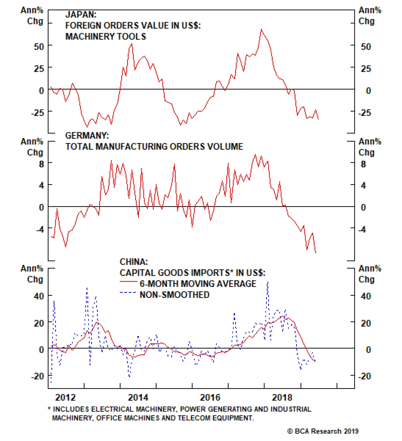
Japanese foreign machinery tool orders and German industrial orders are contracting deeply, and have not improved, not even on a rate-of-change basis. Meanwhile, China’s imports of capital goods are contracting at a double-digit pace. Chinese auto sales…
Only in a scenario of a complete collapse in global growth will the Fed cut rates more than what is currently priced in the market. Yet, this scenario would be dollar bullish. In this case, the dollar’s strong inverse relationship with global growth will…

Dear Client, In lieu of next week’s regular report, we will be bringing you a Special Report featuring a no-holds-barred debate over the economic and financial market outlook among three of BCA’s more bullish strategists (Doug Peta, Rob Robis, and yours truly) and three of the more bearish ones (Anastasios Avgeriou, Arthur Budaghyan, and Dhaval Joshi). Best regards, Peter Berezin, Chief Global Strategist Highlights Slowdowns are much more likely to turn into recessions when significant economic and financial imbalances are present. The U.S. does not currently suffer from any of the three major imbalances that have historically heralded recessions – rapid private-sector debt growth; excessive spending in cyclical sectors such as housing, consumer durables, and business capex; or accelerating inflation. Imbalances are larger abroad, but not to the extent that they will trigger a global recession. The combination of ongoing Chinese stimulus and the lagged effect from lower bond yields will lift global growth during the coming months. The inventory cycle, which is likely to subtract at least one full percentage point from U.S. growth in Q2, will also turn from being a headwind to a tailwind. Stay overweight global equities relative to government bonds over the next 12 months. A rebound in global growth will push down the U.S. dollar later this year, creating an opportunity to increase exposure to European and EM equities. Feature Global Growth At A Critical Juncture The global economy has clearly slowed since early 2018 (Chart 1). So far, much of the weakness has been confined to the manufacturing sector. However, the service sector has softened as well (Chart 2). Chart 1The Global Economy Has Slowed...
The Global Economy Has Slowed...
The Global Economy Has Slowed...
Chart 2...Mostly Due To Another Manufacturing Downturn
...Mostly Due To Another Manufacturing Downturn
...Mostly Due To Another Manufacturing Downturn
Regionally, the U.S. has held up somewhat better than most other economies. Nevertheless, the ISM manufacturing and nonmanufacturing indices have both declined, with the former now flirting with the 50 line. All recessions begin as slowdowns but not all slowdowns end in recessions. As we discuss below, slowdowns are much more likely to morph into recessions when financial and economic imbalances are elevated. We confine our empirical analysis to the U.S., but discuss the global context later in the report. Three Key Recessionary Imbalances Three imbalances, in particular, have often been present at the outset of U.S. recessions (Chart 3): Chart 3What Makes A Slowdown Degenerate Into A Recession: Imbalances
What Makes A Slowdown Degenerate Into A Recession: Imbalances
What Makes A Slowdown Degenerate Into A Recession: Imbalances
Rapid private-sector debt growth: Rising debt lifts aggregate demand.1 Fast debt growth is also often associated with bad lending decisions, which makes economies more vulnerable to adverse shocks. An unsustainably high level of cyclical spending: Cyclical spending includes business and residential investment, as well as spending on consumer durable goods. If spending on these categories is elevated, there is more scope for it to decline when the economy turns down. High and rising inflation. When inflation rises above the Fed’s comfort zone, the central bank normally needs to raise rates into restrictive territory. Fast debt growth is also often associated with bad lending decisions, which makes economies more vulnerable to adverse shocks. Table 1 shows every episode since 1960 when the U.S. economy has slowed significantly. To keep things simple, we define a slowdown as a 10-point drop in the ISM manufacturing index from its recent high. Table 1Episodes Of Significant Economic Slowdown
When Do Slowdowns Turn Into Recessions?
When Do Slowdowns Turn Into Recessions?
Of the 15 slowdowns that we examined, seven culminated in recessions. An average of 2.1 of the three imbalances listed above were visible prior to recessions. However, an average of only 0.9 imbalances were present when a recession failed to materialize. This supports our claim that slowdowns are more likely to turn into recessions when significant imbalances are present. The good news for the U.S. is that it currently does not register any of three imbalances that have typically preceded recessions. Equities reacted very differently in the two cases. When a recession did occur following the start of a slowdown, the S&P 500 declined by an average of 3.6% over the subsequent 12 months. When the slowdown failed to turn into a recession, the S&P rose by an average of 18.3%. In the latter case, the recovery in stocks usually coincided with a swift rebound in the ISM index. The U.S. Is Currently 0 For 3 On The Imbalance Front The good news for the U.S. is that it currently does not register any of three imbalances that have typically preceded recessions. Chart 4Reasons Not To Panic About U.S. Corporate Debt (I)
Reasons Not To Panic About U.S. Corporate Debt (I)
Reasons Not To Panic About U.S. Corporate Debt (I)
Private-Sector Debt While U.S. private nonfinancial debt has edged up slightly as a share of GDP since 2015, it remains well below its 2008 peak. In fact, the current business expansion is the only one in the post-war era where private-sector debt has failed to rise above its previous cycle high. A recent Bank of England study examined 130 recessions across 26 countries. It found private debt growth matters much more for recession risk than the level of debt.2 Granted, the composition of debt also matters: While household debt in the U.S. has fallen over the past decade, corporate debt has risen. As a share of GDP, corporate debt is now at the highest level in the post-war era. That said, despite its recent ascent, the ratio of corporate debt-to-GDP is less than two percentage points higher than it was in 2008. One drawback of comparing debt to GDP is that the former is a stock variable while the latter is a flow variable. A more sensible “apples-to-apples” approach is to look at corporate debt in relation to assets rather than GDP. If one does that, one sees that the ratio of U.S. corporate debt-to-assets is below its post-1980 average and only slightly above its post-1950 average. The interest coverage ratio, which compares the profits that companies earn for every dollar of interest that they pay, is above its historic norm (Chart 4). Corporate sector free cash flow – the difference between profits and spending on such things as labor and capital goods – remains in surplus. Every recession during the past 50 years has begun when the free cash flow balance was in deficit (Chart 5). In contrast to mortgages, which are generally held by leveraged institutions such as banks, most corporate debt is held by entities such as insurance companies, pension funds, mutual funds, and ETFs. Banks hold only 18% of corporate debt, down from 40% in 1980 (Chart 6). Thus, while high corporate debt levels could exacerbate the next recession, they are unlikely to engender it. Chart 5Reasons Not To Panic About U.S. Corporate Debt (II)
Reasons Not To Panic About U.S. Corporate Debt (II)
Reasons Not To Panic About U.S. Corporate Debt (II)
Chart 6Banks Have Reduced Their Exposure To The Corporate Sector
Banks Have Reduced Their Exposure To The Corporate Sector
Banks Have Reduced Their Exposure To The Corporate Sector
Cyclical Spending Unlike a restaurant meal or a vacation, a house, office tower, factory, or automobile will usually retain some value for a while after it is purchased. If spending on cyclical items rises to a high level for an extended period of time, a glut will form, requiring a period of lower production. By contrast, if spending on these items is subdued for a long time, pent-up demand will accumulate, requiring a period of higher production. Recessions can result from either economic overheating or financial market overheating. As a share of GDP, cyclical spending is still far below the peaks observed during past expansions. Just as importantly, today’s low level of cyclical spending follows ten years of even lower spending. As a result, the average age of the U.S. capital stock has increased across almost all categories since 2008 (Chart 7). Most notably, the average age of U.S. homes has risen by nearly five years since 2006, the sharpest increase since the Great Depression. Despite the rebound in residential investment from its recessionary lows, the current level of homebuilding still falls short of what is necessary to keep up with household formation. As a consequence, the vacancy rate has fallen to multi-decade lows (Chart 8). Chart 7The Capital Stock Is Aging
The Capital Stock Is Aging
The Capital Stock Is Aging
Chart 8There Is No Glut Of U.S. Homes
There Is No Glut Of U.S. Homes
There Is No Glut Of U.S. Homes
Inflation Recessions can result from either economic overheating or financial market overheating. Economic overheating was the dominant driver of recessions between the late 1960s to early 1980s. Rising inflation preceded the recessions of 1969-70, 1973-75, as well as the back-to-back recessions in 1980-82. Chart 9The 1990 Recession: A Bit Of Everything
The 1990 Recession: A Bit Of Everything
The 1990 Recession: A Bit Of Everything
Overheating also contributed to the 1990 recession. After peaking in 1982, the unemployment rate fell to 5% in 1989, about one percent below its equilibrium level at the time. Core inflation began to accelerate, reaching 5.5% by August 1990. The Fed initially responded to the overheating economy by hiking interest rates. The fed funds rate rose from 6.6% in March 1988 to a high of 9.8% by May 1989. By the summer of 1990, the economy had already slowed significantly. Commercial real estate, still reeling from the effects of the Savings and Loan crisis, weakened sharply. Defense outlays continued to contract following the collapse of the Soviet Union. The final straw was Saddam Hussein’s invasion of Kuwait, which caused oil prices to surge and consumer confidence to plunge (Chart 9). In contrast to earlier downturns, the last two recessions were more the byproduct of financial excesses: The 2007-09 recession stemmed from the housing crash and the financial crisis it generated; the 2001 recession followed the dotcom bust, which precipitated a steep decline in capital spending. What will the next U.S. recession look like? Given the absence of major financial imbalances, the odds are high that the next recession will be a “retro recession,” featuring classic economic overheating. The fact that the Fed has adopted a risk-based approach to monetary policy, which puts great weight on avoiding a deflationary outcome, only raises the likelihood that inflation will eventually move higher. The good news is that this is unlikely to happen anytime soon. While wage growth has picked up, productivity growth has risen even more. As a result, unit labor costs – the ratio of wages-to-productivity – have actually decelerated over the past 18 months. Unit labor cost inflation tends to lead core inflation by up to one year (Chart 10). Given the absence of major financial imbalances, the odds are high that the next recession will be a “retro recession,” featuring classic economic overheating. As we discussed in our latest Strategy Outlook, the Fed will probably not bring rates into restrictive territory until early 2022. This gives the economy plenty of breathing space.3 The Global Dimension The discussion above has focused on the United States. To some extent, this is unavoidable. Not only is the U.S. still the world’s largest economy, but it remains at the heart of the global financial system. U.S. equities account for over half of global stock market capitalization, up from a third in the early 1990s (Chart 11). The dollar continues to be the preeminent reserve currency. As a result, U.S. financial markets drive overseas markets much more than the other way around. Chart 10No Imminent Threat Of A Wage-Price Inflationary Spiral
No Imminent Threat Of A Wage-Price Inflationary Spiral
No Imminent Threat Of A Wage-Price Inflationary Spiral
Chart 11The U.S. Stock Market Capitalization Is More Than Half Of Global
The U.S. Stock Market Capitalization Is More Than Half Of Global
The U.S. Stock Market Capitalization Is More Than Half Of Global
Chart 12
This does not mean that the rest of the world is irrelevant. The global supply chain now dominates international trade. More than half of all cross-border trade is in intermediate goods (Chart 12). Irrespective of the financial and economic imbalances discussed above, a full-blown trade war would upend the global economy, sending the U.S. and the rest of the world into recession. President Trump’s re-election prospects would plummet if U.S. unemployment rose and the stock market plunged. This is the main reason for thinking that the trade talks will ultimately produce some sort of détente. Nevertheless, a severe deterioration of trade relations remains the biggest risk to our bullish view on risk assets. The fact that financial and economic imbalances are generally larger overseas means that the rest of the world is more vulnerable to adverse shocks. Unlike in the United States, private debt has risen sharply as a share of GDP in several key economies over the past decade (Chart 13). Government debt is also a problem in countries such as Italy that do not have central banks which can function as reliable lenders of last resort.
Chart 13
Chart 14Economies With Frothy Housing Markets Risk Having Deeper Downturns
Economies With Frothy Housing Markets Risk Having Deeper Downturns
Economies With Frothy Housing Markets Risk Having Deeper Downturns
Cyclical spending is fairly elevated in a number of countries. Notably, residential investment stands at near record highs as a share of GDP in Canada, Australia, and New Zealand (Chart 14). Home prices are also quite frothy there. When the global economy falls into recession in two-to-three years, these economies will take it on the chin. Investment Conclusions Notwithstanding the risks noted above, we continue to maintain a bullish outlook on global equities and spread product over the next 12 months. To paraphrase Wayne Gretzky, one should invest on the basis of where the economic data is going, not where it is.4 While global growth remains anemic today, the combination of Chinese stimulus and the lagged effect from lower bond yields will boost activity during the coming months. The inventory cycle, which is likely to subtract at least one full percentage point from U.S. growth in Q2, will also turn from being a headwind to a tailwind. Global equities are not super cheap, but they are not particularly expensive either. The MSCI All-Country World Index trades at 15.3-times forward earnings. Given the ultra-low level of global bond yields, this generates an equity risk premium (ERP) that is well above its historical average (Chart 15). From an asset allocation perspective, one should favor stocks over bonds when the ERP is high. Chart 15AEquity Risk Premia Remain Elevated (I)
Equity Risk Premia Remain Elevated (I)
Equity Risk Premia Remain Elevated (I)
Chart 15BEquity Risk Premia Remain Elevated (II)
Equity Risk Premia Remain Elevated (II)
Equity Risk Premia Remain Elevated (II)
The ERP is especially elevated outside the United States. This is partly because non-U.S. stocks trade at a meager 13.3-times forward earnings, but it also reflects the fact that bond yields are lower overseas. The fact that financial and economic imbalances are generally larger overseas means that the rest of the world is more vulnerable to adverse shocks. As global growth accelerates, the dollar will start to weaken (Chart 16). EM and European equities usually outperform the global benchmark in that environment (Chart 17). We expect to upgrade stocks in these regions later this summer. Chart 16The Dollar Is A Countercyclical Currency
The Dollar Is A Countercyclical Currency
The Dollar Is A Countercyclical Currency
Chart 17EM And Euro Area Equities Outperform When Global Growth Improves
EM And Euro Area Equities Outperform When Global Growth Improves
EM And Euro Area Equities Outperform When Global Growth Improves
Peter Berezin, Chief Global Strategist Global Investment Strategy peterb@bcaresearch.com Footnotes 1 Recall that GDP is a flow variable (how much production takes place every period), whereas credit is a stock variable (how much debt there is outstanding). By definition, a flow is a change in a stock. Thus, credit growth affects GDP and the change in credit growth affects GDP growth. 2 Jonathan Bridges, Chris Jackson, and Daisy McGregor, "Down in the slumps: the role of credit in five decades of recessions," Bank Of England Staff Working Paper No. 659, (April 2017). 3 Please see Global Investment Strategy Strategy Outlook, "Third Quarter 2019 Strategy Outlook: The Long Hurrah," dated June 28, 2019. 4 According to Wayne Gretzky, his father, Walter, once advised him to “skate to where the puck is going, not to where it is.” Strategy & Market Trends MacroQuant Model And Current Subjective Scores
Chart 18
Tactical Trades Strategic Recommendations Closed Trades
Highlights Q2/2019 Performance Breakdown: Our recommended model bond portfolio underperformed the custom benchmark index by -19bps in the second quarter of the year. Winners & Losers: Our below-benchmark overall duration stance expressed through country underweights in the U.S. (-25bps) and Italy (-10bps) hurt Q2 returns. This dwarfed the gains from U.S. corporate bond overweights (+14bps) and selective sovereign bond overweights in Germany, Australia and the U.K. Scenario Analysis For Next Six Months: We are adding credit exposure to our model portfolio, increasing spread product allocations in U.S. high-yield and European corporates. In our Base Case scenario, the Fed is likely to deliver some “insurance” rate cuts in the next few months, but by less than the markets are currently discounting, while global growth momentum will stabilize. The resulting price action will favor relative returns from spread product versus government debt. Feature The first half of 2019 produced a surprising result across the global fixed income universe – practically everything delivered a positive total return. From U.S. Treasuries to Italian BTPs to U.S. investment grade industrial corporates to emerging market hard currency sovereigns, all the year-to-date returns are colored green on your Bloomberg screen. Those returns have occurred despite all the uncertainties that investors have had to navigate during the past three months, from shock Trump tariff tweets to persistent weakness in global manufacturing data to swift dovish turns by global central bankers (rate cuts in Australia and New Zealand, the Fed hinting at easing and the ECB signaling a potential restart of asset purchases). In this report, we review the performance of the BCA Global Fixed Income Strategy (GFIS) model bond portfolio during the eventful second quarter of 2019. We also present our updated scenario analysis, and total return projections, for the portfolio over the next six months. As a reminder to existing readers (and to new clients), the model portfolio is a part of our service that complements the usual macro analysis of global fixed income markets. The portfolio is how we communicate our opinion on the relative attractiveness between government bond and spread product sectors. This is done by applying actual percentage weightings to each of our recommendations within a fully invested hypothetical bond portfolio. Q2/2019 Model Portfolio Performance Breakdown: Credit Overweights Help Limit Damage From Below-Benchmark Duration Chart of the WeekBelow-Benchmark Duration Overwhelms Credit Overweights In Q2/19
Duration Losses Offset Credit Gains In Q1/2019
Duration Losses Offset Credit Gains In Q1/2019
The total return for the GFIS model portfolio (hedged into U.S. dollars) in the second quarter was 2.8%, underperforming the custom benchmark index by -19bps (Chart of the Week).1 The bulk of the underperformance came from the government bond side of the portfolio (-33bps) - a function of our below-benchmark duration tilt and underweight stance on sovereign bonds, both occurring against a backdrop of rapidly falling bond yields (Table 1). Partially offsetting that was the outperformance from our recommended overweights in U.S. corporate debt, which helped the spread product side of our model portfolio outperform the benchmark by +14bps. Table 1GFIS Model Bond Portfolio Q2/2019 Overall Return Attribution
Q2/2019 GFIS Model Bond Portfolio Performance Review: Duration Dominates
Q2/2019 GFIS Model Bond Portfolio Performance Review: Duration Dominates
The bar charts showing the total and relative returns for each individual government bond market and spread product sector are presented in Charts 2 and 3.
Chart 2
Chart 3
The main individual sectors of the portfolio that drove the excess returns were the following: Biggest outperformers Overweight U.S. investment grade industrials (+5bps) Overweight U.S. high-yield Ba-rated (+4bps) Overweight U.S. high-yield B-rated (+4bps) Overweight U.S. investment grade financials (+2bps) Overweight German government bonds with maturity of 7-10 years (+2bps) Biggest underperformers Underweight U.S. government bonds with maturity beyond 10+ years (-10bps) Underweight Italy government bonds with maturity beyond 10+ years (-6bps) Underweight Japanese government bonds with maturity beyond 10+ years (-6bps) Underweight U.S. government bonds with maturity of 1-3 years (-5bps) Underweight U.S. government bonds with maturity of 3-8 years (-5bps) Chart 4 presents the ranked benchmark index returns of the individual countries and spread product sectors in the GFIS model bond portfolio for Q2/2019. The returns are hedged into U.S. dollars (we do not take active currency risk in this portfolio) and are adjusted to reflect duration differences between each country/sector and the overall custom benchmark index for the model portfolio. We have also color-coded the bars in each chart to reflect our recommended investment stance for each market during Q2/2019 (red for underweight, blue for overweight, gray for neutral).2 Ideally, we would look to see more blue bars on the left side of the chart where market returns are highest, and more red bars on the right side of the chart were returns are lowest.
Chart 4
Our underweight tilts on European Peripheral sovereign debt were our biggest “miss” in the quarter, as Spanish and Italian yields plunged after the ECB signaled future rate cuts and a potential return to bond purchases in order to boost flailing European growth. We had been viewing Spain and Italy as growth-focused credit stories rather than yield plays, leaving us to maintain a cautious stand on both markets given worsening economic momentum (but with an imbedded “long Spain/short Italy” tilt by having a smaller relative underweight in Spain). In terms of our best “hits” in the quarter, our overweight stance on U.S. investment grade corporates and Australian government bonds performed relatively well. We also avoided a big “miss” by upgrading emerging market U.S. dollar-denominated sovereign debt to neutral from underweight on April 30.3 We also avoided a bigger hit to the portfolio through tactical adjustments made in late May, when we added back some interest rate duration to the portfolio given the increasing uncertainties from slowing global growth and rising U.S. trade policy hawkishness.4 We also reduced our U.S. corporate bond overweights at the same time, but the additional duration exposure was the more important factor – without those changes, the portfolio would have lagged the benchmark index by another -8bps in Q2. In terms of our best “hits” in the quarter, our overweight stance on U.S. investment grade corporates and Australian government bonds performed relatively well. Bottom Line: Our recommended model bond portfolio underperformed the custom benchmark index in the second quarter of the year, with the drag on performance from underweight exposure to U.S. Treasuries and Italian BTPs overwhelming the gains from credit overweights in the U.S. Future Drivers Of Portfolio Returns Looking ahead, the performance of the model bond portfolio will be driven by two main factors: our below-benchmark duration bias and our overweight stance on global corporate debt versus government bonds. In terms of the specific high-level weightings in the model portfolio, we currently have a moderate overweight, equal to three percentage points, on spread product versus government debt (Chart 5). This reflects a more constructive view on future global growth, with early leading economic indicators starting to bottom out to the benefit of growth-sensitive assets like corporate debt.
Chart 5
That faster growth backdrop will also benefit our below-benchmark duration stance through a rebound in government bond yields. This should happen only slowly, however, as global central bankers are likely to keep their newly-dovish policy bias in place for some time until there are more decisive signs of accelerating growth AND inflation. Chart 6Overall Portfolio Duration: Below-Benchmark
Overall Portfolio Duration: Below-Benchmark
Overall Portfolio Duration: Below-Benchmark
We are maintaining our below-benchmark duration tilt (0.5 years short of the custom benchmark), but we recognize that the underperformance from duration seen in the first half of 2019 will only be clawed back slowly over the next six months (Chart 6). As for country allocation, we continue to favor regions where looser monetary policy is most likely (core Europe, Australia, Japan and the U.K.). We are staying underweight the U.S., however, as the market’s expectations for the Fed are too dovish, with -82bps of rate cuts now discounted over the next twelve months. We are also keeping our underweight stance on Italian government bonds, which we now see as overvalued after the recent rally. We are maintaining our below-benchmark duration tilt (0.5 years short of the custom benchmark), but we recognize that the underperformance from duration seen in the first half of 2019 will only be clawed back slowly over the next six months We are, however, making some adjustments to the portfolio allocations to reflect our expectation of less negative news on global growth and easier monetary policies from global central bankers facing uncertainty alongside too-low inflation expectations: Increasing the overweight to U.S. high-yield corporates, boosting the allocation to Ba-rated and B-rated credit tiers by one percentage point each. This is funded by reducing our U.S. Treasury allocation by two percentage points. Upgrading euro area corporates to overweight, increasing the allocation to both investment grade and high-yield by one percentage point each. This is funded by reducing our German government bond allocation by two percentage points. Upgrading U.K. investment grade corporates to neutral, funded by reducing U.K. Gilt exposure by 0.5 percentage points. Upgrading Spanish government bonds to neutral, funded by reducing German exposure by 0.3 percentage points. These changes will boost the overall spread product allocation to 50% of the portfolio (an overweight of seven percentage points versus the benchmark index). This will also boost the overall yield of the portfolio to 3.2%, +6bps greater than that of the benchmark. That relative yield advantage looks even better in U.S. dollar terms, with currency hedging adding an additional +16bps to the relative portfolio yield given the current powerful carry advantage of the greenback (Chart 7). Chart 7Portfolio Yield: Small Positive Carry
Portfolio Yield: Small Positive Carry
Portfolio Yield: Small Positive Carry
Chart 8Portfolio Risk Budget Usage: Cautious
Portfolio Risk Budget Usage: Cautious
Portfolio Risk Budget Usage: Cautious
Even though we have decent-sized overall tilts on global duration and spread product allocation, our estimated tracking error (excess volatility of the portfolio versus its benchmark) remains low (Chart 8). We remain comfortable with a portfolio tracking error of 38bps, well below our self-imposed 100bps ceiling, as the internal weightings in the portfolio are helping keep overall portfolio volatility at a modest level. Scenario Analysis & Return Forecasts In April 2018, we introduced a framework for estimating total returns for all government bond markets and spread product sectors, based on common risk factors.5
Chart
Chart
For credit, returns are estimated as a function of changes in the U.S. dollar, the Fed funds rate, oil prices and market volatility as proxied by the VIX index (Table 2A). For government bonds, non-U.S. yield changes are estimated using historical betas to changes in U.S. Treasury yields (Table 2B). This framework allows us to conduct scenario analysis of projected returns for each asset class in the model bond portfolio by making assumptions on those individual risk factors. In Tables 3A & 3B, we present our three main scenarios for the next six months, defined by changes in the risk factors, and the expected performance of the model bond portfolio in each case. The scenarios, described below, are all driven by what we believe will be the most important driver of market returns over the rest of 2019 – the momentum of global growth and the path of U.S. monetary policy.
Chart
Chart
Our Base Case: the Fed delivers -50bps of easing by the end of 2019, the U.S. dollar depreciates by -3%, oil prices rise by +10%, the VIX index hovers around 15, and there is a mild bear-steepening of the U.S. Treasury curve. This is a scenario where the Fed delivers a rate cut in July and one more “insurance cut” before year-end, while signaling that no other easing beyond that. The model bond portfolio is expected to beat the benchmark index by +57bps in this case. Global Growth Rebounds: the Fed stays on hold to year-end, the U.S. dollar is flat, oil prices increase +10%, the VIX index falls to 12 and there is a mild bear-flattening of the U.S. Treasury curve. This is a scenario where improving economic data outside the U.S. diminishes the fears of a U.S. recession, allowing the Fed to stand pat and keep rates unchanged as financial market volatility stays muted. The model bond portfolio is expected to outperform the benchmark by +50bps here. Global Downturn Intensifies: the Fed cuts the funds rate by -75bps by year-end, the U.S. dollar falls by -5%, oil prices decline -15%, the VIX index increases to 30 and there is a bull steepening of the U.S. Treasury curve. This is a scenario where U.S./global growth momentum continues to fade, prompting the Fed to deliver a series of curve-steepening rate cuts to try and stabilize elevated financial market volatility amid increasing recession risks. The model portfolio will severely underperform the benchmark by -41bps with this outcome. The scenario inputs for the four main risk factors (the fed funds rate, the price of oil, the U.S. dollar and the VIX index) are different than what was presented in our last model bond portfolio review in mid-April (Chart 9). Then, we were contemplating scenarios involving the Fed keeping rates stable and even potentially looking for an opportunity to deliver another rate hike by year-end. Now, given the Fed’s clear dovish shift after the downshift in global growth momentum, two of our three main scenarios involve rate cuts in the U.S. The only scenario where Treasury yields can fall further, however, is if the global economic downturn deepens – a scenario we view as more of a tail risk rather than a higher-probability possibility (Chart 10). Chart 9Risk Factors Assumptions For The Scenario Analysis
Risk Factors Assumptions For The Scenario Analysis
Risk Factors Assumptions For The Scenario Analysis
Chart 10U.S. Treasury Yield Assumptions For The Scenario Analysis
U.S. Treasury Yield Assumptions For The Scenario Analysis
U.S. Treasury Yield Assumptions For The Scenario Analysis
In terms of our conviction level among the main drivers of the model portfolio returns – duration allocation (across yield curves and countries) and asset allocation (credit versus government bonds) – we are most confident that credit returns will exceed those of sovereign debt over the next six months. In terms of our conviction level among the main drivers of the model portfolio returns – duration allocation (across yield curves and countries) and asset allocation (credit versus government bonds) – we are most confident that credit returns will exceed those of sovereign debt over the next six months. Bottom Line: We are adding credit exposure to our model portfolio, increasing spread product allocation in U.S. high-yield and European corporates. In our Base Case scenario, the Fed is likely to deliver some “insurance” rate cuts in the next few months, but by less than the markets are currently discounting, while global growth momentum will stabilize. The resulting price action will favor spread product over government bonds, helping boost the returns of our model portfolio. Robert Robis, CFA, Chief Fixed Income Strategist rrobis@bcaresearch.com Ray Park, CFA, Research Analyst ray@bcaresearch.com Footnotes 1 The GFIS model bond portfolio custom benchmark index is the Bloomberg Barclays Global Aggregate Index, but with allocations to global high-yield corporate debt replacing very high quality spread product (i.e. AA-rated). We believe this to be more indicative of the typical internal benchmark used by global multi-sector fixed income managers. 2 Note that sectors where we made changes to our recommended weightings during Q2/2019 will have multiple colors in the respective bars in Chart 4. 3 Please see BCA Global Fixed Income Strategy Weekly Report, “It’s Time To Break Out The Fine China”, dated April 30, 2019, available at gfis.bcaresearch.com. 4 Please see BCA Global Fixed Income Strategy Weekly Report, “The Message From Low Bond Yields”, dated May 28, 2019, available at gfis.bcaresearch.com. 5 Please see BCA Global Fixed Income Strategy Weekly Report, “GFIS Model Bond Portfolio Q1/2018 Performance Review: A Rough Start”, dated April 10th 2018, available at gfis.bcareseach.com. Recommendations The GFIS Recommended Portfolio Vs. The Custom Benchmark Index
Q2/2019 GFIS Model Bond Portfolio Performance Review: Duration Dominates
Q2/2019 GFIS Model Bond Portfolio Performance Review: Duration Dominates
Duration Regional Allocation Spread Product Tactical Trades Yields & Returns Global Bond Yields Historical Returns
This will put upward pressure on forward curves, nudging oil near our Commodity & Energy Strategy service’s target of $75 per barrel. Should demand pick up later this year, it will supercharge the uptrend. More importantly, the risk of escalation…
In 2H19, accommodative global monetary policy and fiscal stimulus will revive demand for industrial commodities, particularly in EM economies. This will be most apparent in oil markets, where our Commodity & Energy Strategy team continues to expect demand…
The current global manufacturing recession stems primarily from China. Our Emerging Markets Strategy team's leading indicators of the mainland business cycle suggest that more growth disappointments are likely before China’s growth and other economies’…
Since early this year, our Emerging Markets Strategy team has been arguing that expectations of an early recovery in the Chinese economy and global trade are unwarranted. So far, our baseline economic view has played out – mainland growth has been rather…
Oil prices will remain volatile as markets work through the lingering effects of tighter financial conditions prevailing last year, which, along with extended angst over Sino-U.S. trade tensions, slowed commodity demand growth (Chart of the Week). In 2H19, globally accommodative monetary policy and fiscal stimulus will revive demand for industrial commodities, particularly in EM economies. This will be most apparent in oil markets, where we continue to expect demand growth to strengthen going into 2020, aided in part by a weaker USD. On the supply side, this week’s extension of OPEC 2.0’s production cuts into 1Q20 means growth will remain constrained. Prices will rise, and forward curves, particularly for Brent, will steepen as refiners are forced to draw inventories to meet product demand.1 We continue to expect Brent to average $73/bbl this year and $75/bbl next, respectively. We expect WTI to trade $7/bbl and $5/bbl below that this year and next. Chart of the WeekEasing Financial Conditions Will Spur Oil Demand
Easing Financial Conditions Will Spur Oil Demand
Easing Financial Conditions Will Spur Oil Demand
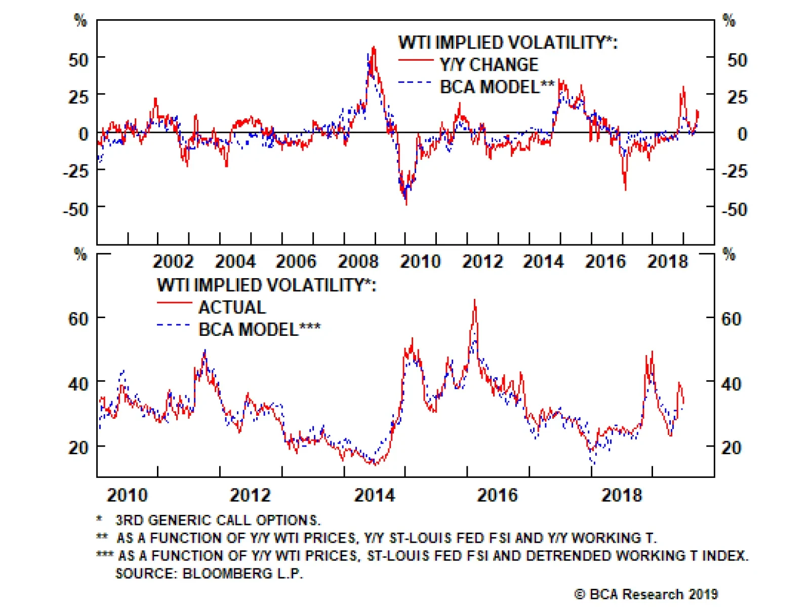
Highlights Energy: Overweight. Venezuela’s oil production reportedly recovered to 1.1mm b/d in June. Most of the increased production found its way to China, which accounted for just under 60% of crude and product exports.2 Given its modus operandi, we believe OPEC 2.0 likely will accommodate higher production in Venezuela by reducing production in other member states, keeping overall output relatively constant. Base Metals: Neutral. Copper treatment and refining charges fell to new lows at the end of last week, with Fastmarkets MB’s Asia – Pacific TC/RC index recording its lowest level on record at $52.40/MT ($0.0524/lb).3 TC/RC levels fall when supplies are low, as refiners have to discount their services to attract concentrate supplies. Elsewhere, workers at Codelco’s Chuquicamata copper mine agreed to a new contract last week, ending a brief strike. Precious Metals: Neutral. Gold’s rally resumed this week, reflecting investors’ expectations for expanded central-bank accommodation globally, which, all else equal, will keep interest rates lower for longer. The Fed's dovish turn, in particular, will weaken the USD later this year, which will be positive for EM commodity demand, the engine for commodity demand growth globally. Ags/Softs: Underweight. The USDA reported 56% of corn in the ground was in good to excellent condition last week, vs. 76% of the crop last year. For soybeans, 54% of the U.S. crop was in good or excellent condition, vs. 71% last year. The USDA’s Crop Progress reports cover 92% and 95% of total acreage planted in the U.S., respectively. Feature Oil prices will remain volatile over the short term, as markets transition from tighter monetary conditions to a more accommodative global backdrop (Chart 2). Based on our research into the drivers of oil-price volatility, this should translate into a less stressful pricing environment for industrial commodities generally, base metals and oil in particular (Chart 3).4 Chart 2Volatility Indicators Are Moderating
Volatility Indicators Are Moderating
Volatility Indicators Are Moderating
Chart 3Signaling Oil Price Volatility Will Fall
Signaling Oil Price Volatility Will Fall
Signaling Oil Price Volatility Will Fall
Much of the current oil-price volatility is being driven by worries over damage to aggregate global demand and growth expectations in the wake of the Sino-U.S. trade war, and by what now appears to be a too-aggressive posture by central banks implementing rates-normalization policies last year. Both of these can affect consumption and investment locally and globally.5 Fear That Real Demand Will Weaken At present, any indication real demand is faltering – e.g., weaker manufacturing PMIs – gives industrial commodities an excuse to sell off (Chart 4). In the case of the Sino-U.S. trade war, presidents Xi and Trump appear to have agreed to re-start trade negotiations. Markets are not going to be terribly concerned with the specifics of a trade deal between the U.S. and China, but it does appear some rollback in U.S. tariffs will be necessary for a trade deal – perhaps in exchange for greater access to Chinese markets. However, our geopolitical strategists make the odds of a trade deal by the time U.S. elections roll around 1:3. Our colleagues in BCA Research’s Global Investment Strategy note, “The specifics of the deal are less important than there being a deal – any deal – that avoids a major escalation. Ultimately, the distinction between a ‘small’ trade war and a ‘moderate’ trade war is a function of how high tariffs end up being. Tariffs are taxes, and while no one likes to pay taxes, they are a familiar part of the global capitalist system.”6 As for monetary policy, major central banks are embarked on a coordinated effort to reverse falling inflation expectations, and will be vigorously stimulating their money supply and credit growth over the balance of the year. In addition, fiscal stimulus globally – in the U.S. and China most prominently – will boost real demand for industrial commodities, particularly oil and base metals.7 Monetary and fiscal stimulus operates with a lag, which is why we continue to expect its more visible for commodity demand to become apparent in commodity prices later in 2H19 and next year. This lagged effect can be seen in our expectation for the evolution of EM import volumes to year end, which we estimate using data compiled the CPB World Trade Monitor (Chart 5). EM import volumes are closely tied to the evolution of EM income, which drives global commodity demand.8 Chart 4Globally, The Real Economy Has Slowed
Globally, The Real Economy Has Slowed
Globally, The Real Economy Has Slowed
Chart 5EM Imports and Income Will Rebound
EM Imports and Income Will Rebound
EM Imports and Income Will Rebound
In our modeling of supply-demand balances and prices, we accounted for the reduced EM GDP growth brought about by more restrictive monetary policy last year and the slowdown in global trade in our most recent forecast. In our base case, we took our expected global oil-demand growth this year down to 1.35mm b/d from 1.5mm b/d earlier, and to 1.55mm b/d next year from 1.6mm b/d previously. These adjustments reduced our price expectation for Brent crude oil slightly to $73/bbl this year and $75/bbl next year, with WTI trading $7/bbl and $5/bbl below those respective levels (Chart 6). Chart 6Our Forecasts Reflect Lower Demand, Tighter Supply
Our Forecasts Reflect Lower Demand, Tighter Supply
Our Forecasts Reflect Lower Demand, Tighter Supply
Oil Markets Will Get Tighter For all of the concern over real demand, prompt demand remains stout relative to available supply, as can be seen in the backwardations for global benchmark crude oil prices (Chart 7). This week’s extension of OPEC 2.0’s production cuts into 1Q20 means supply growth will remain constrained, which, given our demand expectation, will tighten balances globally (Chart 8).9 Chart 7Global Oil Benchmarks Remain Backwardated
Global Oil Benchmarks Remain Backwardated
Global Oil Benchmarks Remain Backwardated
Chart 8Oil Supply Demand Balances Will Tighten
Oil Supply Demand Balances Will Tighten
Oil Supply Demand Balances Will Tighten
Chart 9Oil Inventories Will Fall, As Supply Is Constrained
Oil Inventories Will Fall, As Supply Is Constrained
Oil Inventories Will Fall, As Supply Is Constrained
As balances tighten in the wake of global fiscal and monetary stimulus, oil prices will rise, and forward curves, particularly for Brent, will steepen as refiners are forced to draw inventories to meet product demand (Chart 9). For this reason we remain long September – December 2019 Brent vs. short September – December 2020 Brent, expecting backwardation to increase.10 Bottom Line: We remain constructive toward oil markets, as they transition to a more accommodative monetary backdrop globally. Combined with fiscal stimulus in the U.S. and China in particular, demand will remain supported in 2H19 and 2020. The extension of OPEC 2.0’s production-cutting deal will tighten markets, forcing refiners to draw down inventories. Robert P. Ryan, Chief Commodity & Energy Strategist rryan@bcaresearch.com Footnotes 1 OPEC 2.0 is a name we coined for the OPEC/non-OPEC oil-producing coalition led by the Kingdom of Saudi Arabia (KSA) and Russia. Their agreement to extend production cuts of 1.2mm b/d into 1Q19 was announced this week in Vienna. Please see OPEC/non-OPEC rolls over oil output cuts for 9 months published by S&P Global Platts on July 2, 2019. Compliance with these cuts has been higher by ~ 400k b/d in 1H19 by our reckoning. 2 Please see Venezuela's June oil exports recover to over 1 million bpd: data published July 2, 2019, by reuters.com. 3 Please see Copper concs TCs drop marginally on traders purchase; Cobre Panama’s fresh supply hits market published by Fastmarkets MB June 28, 2019. 4 We are using “volatility” in the technical sense here – i.e., the standard deviation of per-annum returns. We have shown this can be explained by different variables, including EM volatility; U.S. financial conditions – as seen in the St. Louis Fed’s financial-stress index; and by speculative positioning, which tends to follow the evolution of prices as news flows change. For discussions of our volatility modeling, including the construction of Working’s T index, please see Specs Back Up The Truck For Oil, published April 26, 2018, and Feedback Loop: Spec Positioning & Oil Price Volatility, published May 10, 2018, by BCA Research’s Commodity & Energy Strategy. Both are available at ces.bcaresearch.com. 5 Please see The economic implications of rising protectionism: a euro area and global perspective published by European Central Bank April 24, 2019. 6 Please see Third Quarter 2019 Strategy Outlook: The Long Hurrah, BCA Research’s global macro outlook for 3Q19, published June 28, 2019, by our Global Investment Strategy. It is available at gis.bcaresearch.com. The larger issues that will have to be addressed at some point in the future are non-tariff barriers to trade, exemplified by Huawei’s exclusion from access to U.S. technology on national security grounds. An expansion of such non-tariff barriers would strand huge amounts of capital globally, which likely would lead to a global recession. 7 Our chief global strategist, Peter Berezin, notes in the above-cited BCA Research third-quarter outlook that Fed policy is expected to remain ultra-accommodative into late 2021, which will push the USD lower later this year, and will support commodity demand generally. 8 We use an FX-based model to estimate EM import volumes to year end off the CPB data. 9 We will be updating our Venezuela and OPEC 2.0 production estimates to reflect this development in our July global oil market balance publication later this month. 10 We have been long 2H19 Brent vs. short 2H20 Brent since February 28, 2019. The July and August pieces of this position returned 222.7% and 273% since inception. We remain long the September – December exposure. Investment Views and Themes Recommendations Strategic Recommendations TRADE RECOMMENDATION PERFORMANCE IN 2019 Q2
Image
Commodity Prices and Plays Reference Table Trades Closed in 2019 Summary of Closed Trades
Image
Highlights The EM equity and currency rebounds should be faded. When corporate profits are contracting, lower interest rates typically do not preclude equity prices from dropping. This is the case in EM and China. Our leading indicators for the Chinese business cycle continue to point to intensifying profit contraction in both China and EM. The ratio of global broad money supply to the current value of securities worldwide is at an all-time low. This casts doubt on the “too much money chasing too few assets” hypothesis. Feature Chart I-1EM Share Prices: Decision Time
EM Share Prices: Decision Time
EM Share Prices: Decision Time
EM share prices are at a critical juncture (Chart I-1). Their ability to hold their recent lows and break above their April highs will signify that a sustainable cyclical rally is in the making. Failure to punch through April’s highs will pose a major breakdown risk. In brief, EM is facing a make-it-or-break-it moment. Fundamentally, the outlook for EM risk assets and currencies largely hinges on economic growth in general and corporate profits in particular. In our June 20 report, we illustrated that the primary drivers of EM risk assets and currencies have historically been their business cycles and profit growth – not U.S. interest rates. Falling interest rates are positive for share prices when profits are expanding, even if at a slower rate. However, when corporate profits are contracting, lower interest rates typically do not preclude equity prices from dropping. Hence, lower global interest rates in of themselves are not a sufficient condition to foster a sustainable cyclical EM rally. As to EM corporate profits, the rate of their contraction will continue deepening. Since early this year, we have been arguing that expectations of recovery in the Chinese economy and global trade are unwarranted. That is why BCA’s Emerging Markets Strategy team contends that EM risk assets and currencies, as well as China-plays, face the risk of a breakdown. This differs from BCA’s house view, which is positive on global risk assets in general. Global And Chinese Business Cycles: No Recovery So Far Chart I-2Chinese A-Share EPS Is Heading Into Contraction
Chinese A-Share EPS Is Heading Into Contraction
Chinese A-Share EPS Is Heading Into Contraction
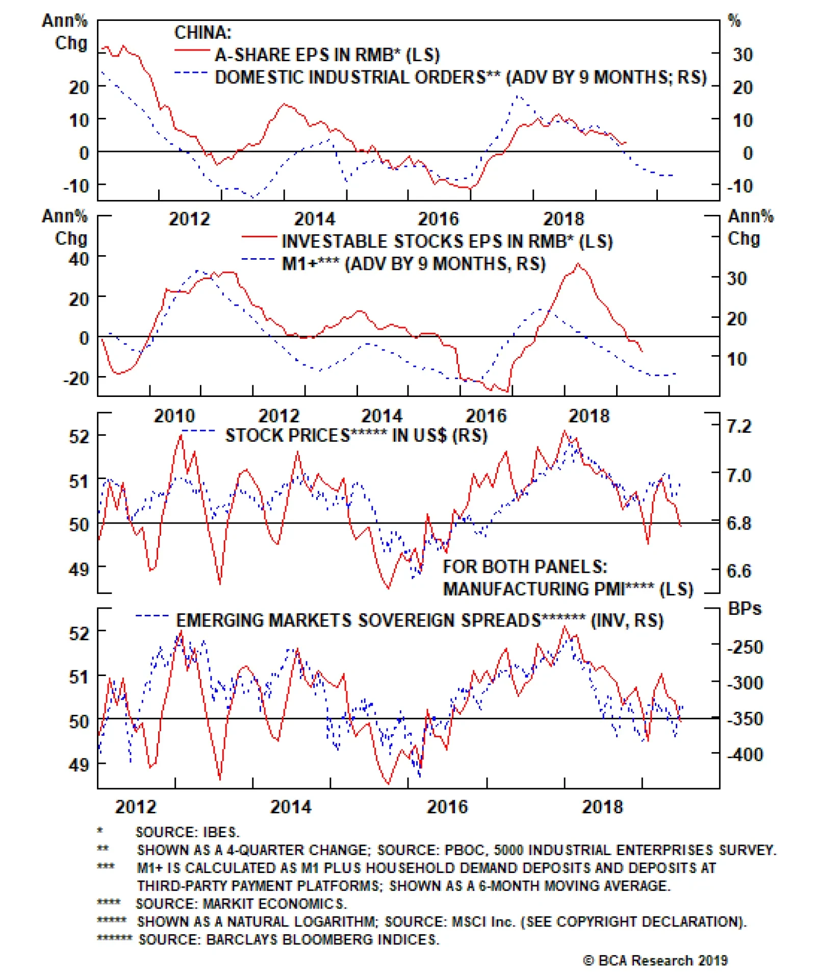
The rebound in EM risk assets and currencies since last December has occurred despite no improvement in both China’s business cycle and global trade, and despite the deepening contraction in EM corporate profits. Since early this year, we have been arguing that expectations of recovery in the Chinese economy and global trade are unwarranted. So far, our baseline economic view has played out – mainland growth has been rather weak, and global trade has contracted. Yet EM financial markets have done better than we had anticipated. China’s domestic industrial new orders lead Chinese A-share earnings per share growth rate by about nine months and point to intensifying profit slump into early 2020 (Chart I-2). Furthermore, China’s adjusted narrow money(M1+)1 growth leads Chinese investable stocks earnings per share (EPS) by about nine months, and is also pointing to further compression (Chart I-3). Finally, Korea’s exports are shrinking, as are EM EPS (Chart I-4, top panel). Chart I-3Chinese Investable Companies' EPS Is Already Shrinking
Chinese Investable Companies' EPS Is Already Shrinking
Chinese Investable Companies' EPS Is Already Shrinking
Chart I-4Korean Exports And EM EPS
Korean Exports And EM EPS
Korean Exports And EM EPS
Notably, both Korean exports values and EM EPS in U.S. dollars terms are on par with their early 2011 levels (Chart I-4, bottom panel). This indicates that neither Korean exports nor EM EPS have expanded sustainably over the past eight years. Chart I-5Global Stocks Did Not Lead Global PMI Historically
Global Stocks Did Not Lead Global Manufacturing PMI Historically
Global Stocks Did Not Lead Global Manufacturing PMI Historically
Is it possible that the current gap between global share prices and global manufacturing is due to the fact that financial markets are forward-looking and lead business cycles? Historical evidence suggests that global share prices have not led the global manufacturing PMI, as exhibited in Chart I-5. In fact, global share prices have actually been coincident with the global manufacturing PMI not only throughout this decade but before that as well. The de-coupling between share prices and the manufacturing PMI is currently also present in EM, albeit in a less-striking form. Chart I-6 illustrates that the EM manufacturing PMI has slipped below 50 line, yet share prices have recently rebounded and sovereign spreads have tightened. In a nutshell, the divergence between global share prices and the global manufacturing PMI is unprecedented. This cannot be explained by falling global bond yields either. The latter were falling in the previous business cycle downtrends (2011-12 and 2015), yet share prices did not deviate from the global manufacturing PMI during those episodes (Chart I-5). Chart I-6EM PMI And EM Risk Assets
EM PMI And EM Risk Assets
EM PMI And EM Risk Assets
Chart I-7The Rest Of World's Exports To China Will Continue Shrinking
The Rest Of Worlds' Exports To China Will Continue Shrinking
The Rest Of Worlds' Exports To China Will Continue Shrinking
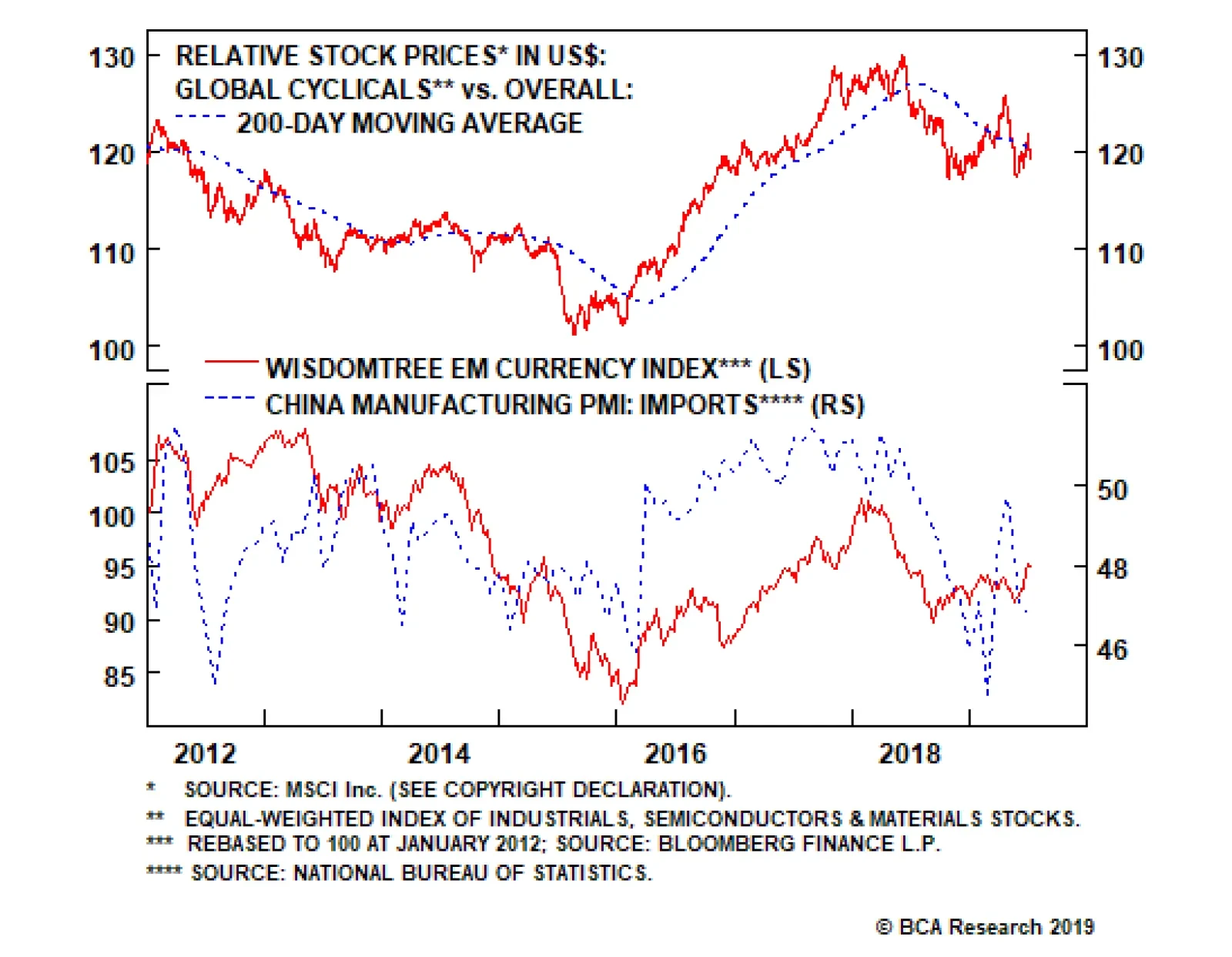
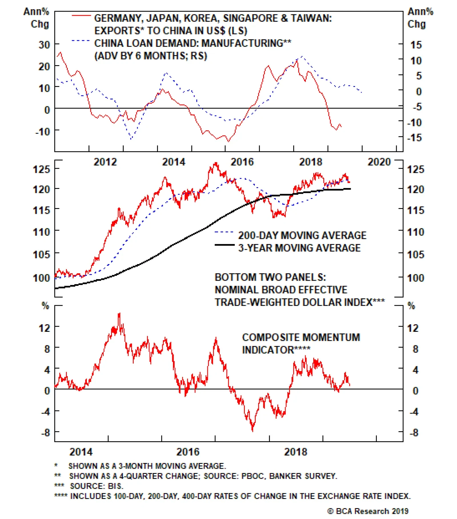
It seems that the global equity and credit markets expect an imminent recovery in the global business cycle in general and in China in particular. As we elaborated in the previous reports, the current global manufacturing recession stems primarily from China. Our leading indicators of the mainland business cycle suggest that more growth disappointments are likely before China’s growth and other economies’ shipments to the mainland hits a bottom (Chart I-7). For example, Korea’s exports to China in June were still dropping by 24% from a year ago. The primary reason for the lack of revival in growth is that China’s stimulus efforts have so far not been large enough, and the marginal propensity to spend among households and companies is diminishing, offsetting the positive effect of the stimulus, as we have discussed in previous reports. Will the recent G20 trade truce between the U.S. and China boost business confidence worldwide and in China? In our view, it is unlikely to produce a quick and meaningful recovery in business confidence among multinational companies and Chinese businesses. Corporate managers have probably come to realize that the U.S.-China row is not about import tariffs but rather geopolitical confrontation between the existing hegemon and a rising superpower. Hence, there is no easy solution that will satisfy both parties. An acceptable resolution for China will be unacceptable for the U.S., and vice versa. Hence, it will be hard to find a formula that gratifies both sides politically and economically. Overall, we reckon there are low odds in the next six months of an agreement between the U.S. and China that removes tariffs, addresses structural issues and satiates both nations. Korea’s exports are shrinking, as are EM EPS. Finally, even though the S&P 500 is hovering around its previous highs, under-the-surface dynamics have been less upbeat. Specifically, the equal-weighted share price index of U.S. high-beta stocks in cyclical sectors such as industrials, technology and consumer discretionary versus the S&P 500 has been tame and has not yet broken above its 200-day moving average (Chart I-8, top panel). The same holds true for the relative performance of an equal-weighted stock index of global cyclical sectors such as industrials, materials and semiconductors against the overall global equity benchmark (Chart I-8, bottom panel). Conversely, despite its recent setback, the U.S. dollar has technically not yet broken down (Chart I-9, top panel). In fact, our composite momentum indicator for the broad trade-weighted dollar has troughed at zero – a sign that downside is limited and another up-leg will likely emerge soon (Chart I-9, bottom panel). Chart I-8Cyclical Stocks Have Been Underperforming
bca.ems_wr_2019_07_04_s1_c8
bca.ems_wr_2019_07_04_s1_c8
Chart I-9The U.S. Dollar Has Technically Not Broken Down
The U.S. Dollar Has Technically Not Broken Down
The U.S. Dollar Has Technically Not Broken Down
Bottom Line: The EM equity and currency rebounds should be faded. As EM currencies depreciate, sovereign and corporate credit spreads will likely widen. Asset allocators should continue underweighting EM equities and credit markets relative to their DM peers. Too Much Money Chasing Too Few Assets? Many investors identify “liquidity” as the main reason why global equity and credit markets have done so well this year, despite the relapsing global business cycle. Yet there are as many definitions of “liquidity” as there are investors. Many commentators use the term “liquidity” to denote balance sheet expansion by global central banks. As part of their quantitative easing programs, central banks in the U.S., U.K., Japan, the euro area, Switzerland and Sweden have expanded their balance sheets enormously. In line with their asset expansion, their liabilities – the monetary base, consisting primarily of commercial banks’ excess reserves – have also mushroomed. Nevertheless, broad money supply has grown only modestly in these economies.2 The principal reason behind this phenomenon has been a collapse in the money multiplier due to both banks’ unwillingness to boost lending proportionally to their swelling excess reserves, and a persistent lack of demand for credit among households and businesses. This computation casts doubt on the “too much money chasing too few assets” hypothesis. Broad money supply includes all types of deposits at commercial banks and cash in circulation. Crucially, it does not include commercial banks’ excess reserves at central banks. This differentiation between broad money and excess reserves at central banks is vital because excess reserves are not used to purchase goods, services or assets/securities. Hence, a true measure of purchasing power for assets, goods and services is broad money supply. Consistently, the pertinent liquidity ratio for financial markets can be computed by dividing global broad money supply by the value of all securities outstanding excluding those owned by central banks. The top panel of Chart I-10 depicts the ratio of the sum of broad money supply in 12 economies3 - excluding China - to the market value of investable global equities and bonds. The latter is calculated as the market cap of the Datastream World Equity Index plus the market value of the Barclays Aggregate Bond Index, excluding securities owned by central banks (Chart I-11). Bonds include both government and corporate issues. Chart I-10Comparing Global Broad Money And Market Value Of Outstanding Securities
Comparing Global Broad Money And Market Value Of Outstanding Securities
Comparing Global Broad Money And Market Value Of Outstanding Securities
Chart I-11Broad Money, Securities Absorbed By QEs And Value Of Outstanding Securities
Broad Money, Securities Absorbed By QE And Value Of Outstanding Securities
Broad Money, Securities Absorbed By QE And Value Of Outstanding Securities
We exclude China from this calculation because its money supply (deposits) is not internationally “mobile” – i.e., due to capital controls, Chinese residents cannot convert their renminbi deposits to other currencies, or use them to purchase international securities. Likewise, we exclude Chinese on-shore equity and bond markets from the calculation because they are not easily accessible to all foreign investors. This broad money supply-to-asset values ratio can be regarded as a rough proxy for available liquidity for financial markets.4 Our interpretation is that a lower ratio means investors have lower cash balances relative to the value of financial assets they hold, and vice versa. Interestingly, the ratio of global broad money to the current value of securities worldwide is at an all-time low (Chart I-10, top panel). Hence, this computation casts doubt on the “too much money chasing too few assets” hypothesis. By flipping this ratio, we compute the ratio of market value of all investable securities (excluding the ones owned by central banks) to broad money supply (Chart I-10, bottom panel). It is at all-time high entailing that the market value of globally investable publically-traded securities has expanded much more than global broad money supply/deposits. Bottom Line: We recognize that this is a simplistic macro exercise, and a more comprehensive methodology is required to compute global cash balances that are available to purchase securities worldwide. However, at minimum the above casts doubt on the hypothesis that “too much money is chasing too few assets”. Arthur Budaghyan Chief Emerging Markets Strategist arthurb@bcaresearch.com Footnotes 1 M1+ is calculated as M1 plus household demand deposits and deposits at third-party payment platforms. 2 Note that when a central bank purchases securities from commercial banks, this operation originates excess reserves, but not a new deposit at commercial banks. However, when a central bank acquires securities from a non-bank entity, such as a pension fund or an insurance company, this transaction creates both excess reserves and a bank deposit that did not exist before. Hence, QE programs have created some deposits but less so than excess reserves. 3 Economies included into this aggregate are the U.S., the euro area, the UK, Japan, Canada, Australia, Switzerland, Sweden, Korea, Taiwan, Hong Kong and Singapore. 4 This calculation does not strip out transactional demand for money, i.e., how much money is required to finance regular economic activity. Given transactional demand for money is not stable, it is hard to estimate and adjust for it. Equity Recommendations Fixed-Income, Credit And Currency Recommendations
Chart I-