Global

Highlights Investors have piled into private equity (PE) in recent years, pushing assets under management (AUM) up to an all-time high of $3 trillion. However, there are increasing concerns about the outlook for the asset class over the next few years. In this report, we look at the fundraising and deal environment for PE, analyze historical risk-adjusted returns in comparison to traditional assets, and suggest how investors can optimize their PE allocation. Private equity and its two major sub-categories, buyouts and growth capital, have generated annualized returns of 13.4%, 13.7%, and 15.0% respectively over the past 32 years, significantly beating the returns from global equities and small-cap stocks of 8.4% and 9.1%. But the current environment is tougher. Dry powder (funds raised but not yet invested) exceeds $1 trillion. PE managers face increased competition from other investors and from companies with large cash balances looking to make acquisitions. Funds raised at the peak of bull markets have a higher probability of underperforming. The next two vintage years (2018 and 2019) face headwinds to making good returns, because of high entry valuations and a rising cost of borrowing. Manager selection is critical for a successful private-equity program. Top-quartile PE funds have outperformed second-quartile funds by as much as 8% a year over the past two decades. Feature Introduction The private equity (PE) market has grown more than five-fold since 2000, lifting assets under management from $577 billion to $2.97 trillion. However, its share of the private investment market has declined from 82% to 58% (Chart 1). Private equity and venture capital investing is said to date back to 1901 when J.P. Morgan purchased Carnegie Steel Co from Andrew Carnegie and Henry Philips for $480 million. The industry has evolved significantly over the years, and now encompasses a wide range of sub-strategies, offering investors a spectrum of exposures with very different risk/return profiles. Chart 1Private Equity Is A $3 Trillion Market
Private Equity: Have We Reached The Top?
Private Equity: Have We Reached The Top?
Compared to public equity, private equity investing is harder because of: 1) long-term illiquidity, whereas public equities can be bought and sold quickly, 2) limited information on target companies, 3) the lack of a clear price discovery function, meaning that pricing in private markets depends heavily on negotiations, 4) less separation between ownership and control - finance providers in PE tend to be managers too. The PE space has matured over the years, and this is clearly seen in the compression of returns. However, many investors remain bullish on this asset class because of its historically attractive risk-adjusted return, and ability to diversify traditional portfolios. As of mid-2017, the median net return of the PE holdings of public pensions globally over the previous 10 years was 8.5% compared to 4.2% for public equities, 4.5% for real estate, and 5.2% for fixed income.1 In this report, we analyze in detail the PE market, with an overview of the fundraising cycle, deal environment, and exit channels. We include in-depth analysis of historical returns from the private equity market in aggregate, and from its two largest sub-categories, buyouts and growth capital. We end by listing the key risks for limited partners (LPs - the investors in PE funds), and include a brief note on private-equity secondary investing. Our key conclusions are: Private equity, including buyouts and growth capital, has had exceptionally good returns over the past three decades, but has been on a structural downtrend as competition has increased. Buyout funds generate a negative skew and moderate kurtosis, whereas growth capital tends to have a larger kurtosis and positive skew. Funds raised at the peak of bull markets have a greater probability of underperforming given their higher entry valuations. This is likely to be the case for funds raised over the next 18 months. The current economic cycle has produced fewer home-run deals - in 2002-2005, 35% of deals produced returns of 3x invested capital, but this fell to 20% in the 2010-2013 period. Megacap buyout funds produce the best returns, but this comes with significantly higher volatility pushing down the risk-adjusted return. These larger funds experience larger negative skew and kurtosis driven by greater use of leverage. Entry valuations of investments made by PE funds have been steadily rising, and so has leverage: the median debt/EBITDA has reached 5.5x. As multiples keep rising, general partners (GPs - the fund managers) have to make up the difference with equity infusion. Top-quartile managers have significantly outperformed. Third-quartile managers struggled even to outperform global equities, and fourth quartile managers failed to preserve their initial capital. The secondary PE market is growing. It provides access to mature portfolio assets deeper into their distributions phase, which reduces the duration of the LP's investment. Fundraising, Deals, And Exits Private equity investing consists of many different sub-categories (Chart 2) that differ in value creation techniques and the maturity of target companies. Buyouts and growth capital are over 90% of the total. Buyouts2 invest in established companies, usually with the intention of improving operations and financials. There is usually substantial use of leverage. Growth capital3 takes significant minority positions in profitable yet still maturing companies mostly without the use of leverage. Secondary funds acquire stakes in PE funds from other LPs. Co-investment funds make minority investments alongside a buyout, recapitalization, or any other non-controlling investment. Turnaround funds aim to revitalize companies that face operational difficulties. Chart 2Buyouts & Growth Capital Are 90% Of PE
Private Equity: Have We Reached The Top?
Private Equity: Have We Reached The Top?
Private-equity firms raised $701 billion in 2017, making the past five years the strongest period for fundraising in history, with a total of $3.2 trillion (Chart 3). Additionally, more than two-thirds of the funds which closed in 2017 met or exceeded their target amounts, and 39% took less than a year to close. The last time fundraising peaked was in 2008, right in the middle of the last recession. However, since 2009, fundraising for buyouts has dropped from 85% to 70% of the aggregate for private equity, with growth capital picking up the slack, rising from 8% to 21%. As fundraising has gotten stronger, PE firms have been raising larger funds.4 These megafunds (with AUM greater than $5 billion) raised $174 billion in 2017, or 58% of that year's total buyout volume, a steep increase from $90 billion in 2016. For investment institutions with large amounts of capital to deploy, megafunds are an attractive and efficient outlet. Another reason for the very strong fundraising environment has been quick follow-up funds, where GPs race to launch new funds before predecessor funds have matured. Historically GPs have waited an average of 62 months between closing one fund and starting the next, but this has come down to 40 months in the past five years. With fundraising so strong, GPs are under pressure to deploy this capital wisely. Global PE deal volume increased by 14% in 2017, surpassing $1.2 trillion (Chart 4). But global deal count has been on the decline since 2015. Along with larger funds being raised, the average deal size in the private market has been rising steadily since the Global Financial Crisis (GFC). Despite increasing deal activity, the sheer volume of fundraising in recent years has led to massive accumulation of dry powder,5 which currently stands at $1.03 trillion. After 2008, dry powder as a percentage of AUM (Chart 5) was on a downward trend because of increased acquisition activity due to attractive valuations following the GFC. But this bottomed in 2012 at 29% and had risen to 35% at the end of 2017. If this level of dry powder accumulation continues, GPs will be forced to reduce hurdle rates and deploy capital into less attractive deals. Chart 3$3.2 Trillion Raised in 5 Years
$3.2 Trillion Raised In 5 Years
$3.2 Trillion Raised In 5 Years
Chart 4Rising Deal Size
Rising Deal Size
Rising Deal Size
Chart 5Harder To Find Attractive Deals
Harder To Find Attractive Deals
Harder To Find Attractive Deals
Another reason for dry powder accumulation is increasing competition for deals both within the private equity market, and from external sources. The number of private equity funds is at an all-time high of 7,775.6 The external competition comes largely from corporate buyers with large cash balances looking for inorganic growth. Corporations have two advantages over PE firms: 1) potential built-in synergies when it comes to integrating the target, giving them the ability to pay a higher price, and 2) a lower cost of capital. An increasing number of corporations have been setting up corporate venture-capital units (Chart 6) to focus on acquisition-led growth. In 2017, there were 38,479 companies bought and sold globally for a total value of $3.3 trillion. But, private equity's share of this market was just 13% by deal value and 8% by deal count (Chart 7). Looking forward, PE funds are likely to act more aggressively and take a larger share of the market, as they did in 2006-2007. In order to increase their share of global deal activity, private-equity funds need to look at more strategic ways to pick up assets: Chart 6Corporations Setting Up VCs
Corporations Setting Up VCs
Corporations Setting Up VCs
Chart 7Buyouts Only A Tiny Player In Global M&A
Private Equity: Have We Reached The Top?
Private Equity: Have We Reached The Top?
Zombie Assets: Assets (portfolio companies) belonging to funds that last raised initial capital between 2003 and 2008 but have not executed a deal since 2015. Currently there are over 100 such companies that are possible targets for takeover in 2018-2019. Carve-Outs: Over the past few years, one in five deals in the U.S. has come from corporations disposing of non-core assets.7 This provides a steady deal flow for buyout and turnaround funds. Public To Private: As multiples in private markets converge with those in public markets, more and more publicly listed companies are being taken private, and this market has doubled since 2016 (Chart 8). Additionally, lenders have become more comfortable about financing these high-value transactions. Buy & Build/Add-Ons: Purchasing cheaper small assets and adding them to existing large established platform companies. This in turn transforms a group of smaller companies at lesser multiples into a larger corporation with a premium valuation. Add-ons made up one-third of deals a decade ago, but that has now reached 50%. But, since such deals are smaller in terms of dollar value, they make up less than 25% of the total deal volume. Finally, PE firms have also been increasing the holding period of the assets in their portfolio. The median holding period before the GFC was four years, and this has now increased to over five years (Chart 9). Additionally, private equity firms exited 40% of all deals in fewer than three years, but now these quick-flips have fallen to only 20%. This is partly a response to increased competition: GPs are skeptical about finding new attractive deals, and this forces them to hold onto assets for as long as possible. Additionally, the new U.S. tax code has increased from one to three years the threshold period for carry to be treated as capital gain with a lower tax rate, rather than taxed as ordinary income. With fundraising on fire but deal activity struggling to keep pace, the final pillar for a successful private equity program is the exit environment. Global PE-backed exits have been flat for the past two years at around $500 billion, with the deal count between 2,500 and 3,000 (Chart 10). The rise in exit activity in 2015 was fuelled by PE firms looking to exit portfolio companies acquired before the financial crisis. By 2017, the dynamic had changed since more than 80% of exits that year were companies acquired in 2009 or later. Finally, dividend recapitalizations8 reached $42 billion in 2017, but these are heavily dependent on an accommodative debt market and positive environment for high-yield bonds. With rising rates, dividend recapitalization, and other forms of special dividends or distributions that require borrowing, become harder to execute. Chart 8Public-To-Private Activity
Public-To-Private Activity
Public-To-Private Activity
Chart 9Longer Holding Periods
Longer Holding Periods
Longer Holding Periods
Chart 10Global PE Exits Are Healthy
Global PE Exits Are Healthy
Global PE Exits Are Healthy
Historical Returns Before we look at the past risk-return profile of investing in this asset class, a note on the data used in this report. All return data are based on the Cambridge Associates Private Investment Benchmarks.9 We are satisfied with the methodology used and the format in which the returns are presented. The provider has taken sufficient steps to minimize survivorship bias. For more details on the data methodology, please see the Appendix. What can investors expect in terms of risk-return exposure from this asset class? Looking at Table 1, private equity and its sub-strategies have comfortably outperformed global equities, with lower volatility, over the past 32 years. Even after statistically adjusting returns for stale pricing,10 volatility for aggregate private equity and buyouts remains lower than for global equities and small-cap stocks. On the other hand, growth capital has had realized volatility greater than that of global equities, but with a significantly higher return; it is still the more attractive investment on a risk-adjusted basis. However, the significantly lower realized volatility of PE in aggregate, and buyout funds in particular, compared to growth capital makes them more attractive investments. Additionally, venture capital experienced volatility of close to 42%, more than double that of small-cap stocks, making it very unattractive from a risk-adjusted perspective. Table 1Risk-Return Spectrum
Private Equity: Have We Reached The Top?
Private Equity: Have We Reached The Top?
However, comparing the performance of PE with that of publicly traded assets could be misleading given the uncertain timing of cash inflows and outflows from private equity programs. Therefore, we also show the Public Market Equivalent11 (PME) to adjust public-market indices for uncertain cash flow streams. Looking at Tables 2-4, we can see that private equity still outperforms equity indices on a PME basis over different time frames. Table 2Private Equity PME Analysis
Private Equity: Have We Reached The Top?
Private Equity: Have We Reached The Top?
Table 3Buyout PME Analysis
Private Equity: Have We Reached The Top?
Private Equity: Have We Reached The Top?
Table 4Growth Capital PME Analysis
Private Equity: Have We Reached The Top?
Private Equity: Have We Reached The Top?
Another unique characteristic of private-market returns is the J-curve effect where investments in private markets take time to bear fruit, and fees are initially based on committed capital rather than invested capital. In addition, the biggest cash flows will be received towards the end, so the returns for the first few years can be misleading. IRR will remain negative until the point when distributions at least match contributions (the payback point). Given the non-linear return distribution of alternative assets such as PE and venture capital, risk analysis is not complete without skewness and kurtosis. Investing in buyout funds generates a negative skew and a moderate level of kurtosis, which means that investors can expect more stable, predictable returns, closer to a normal distribution. However, growth capital tends to have larger kurtosis and positive skew, thereby a higher probability of large upside gains. Since buyout capital structures tend to be more heavily geared, there is a higher skew towards negative returns driven by the leverage effect. Venture capital exhibits a return distribution similar to growth capital, where a few portfolio companies produce large positive returns given the start-up nature of its targets. PE returns remain attractive but, as with other alternative asset classes, performance has been on a downward trend (Chart 11) driven by increased competition. In the 1980s and 1990s, buyout firms exploited the poor performance of large U.S. conglomerates by acquiring underperforming divisions and using leverage. In the early 2000s, funds took advantage of the stock market rise, fuelled by low rates and levered returns. Within the structural downtrend in returns, PE has had a cyclical profile just like public equities. During bull markets there are more exits at higher valuations, and larger distributions to LPs. However, funds raised in bull markets have a higher probability of underperforming given their higher entry valuations. Looking forward, funds from recent vintages that are halfway through their life are likely to be able to take advantage of current tailwinds to build value and exit at the top. However, funds raised in the next two years will have to deal with high entry valuations and a possible increase in the cost of borrowing. There have been fewer write-offs and deals with capital impairments in the post-2009 period than in the years after the 2001 recession. However, the current economic cycle has produced fewer of the home-run deals that really drive PE performance. For example, in 2002-2005, 35% of deals produced returns of 3x invested capital or better, and more than 50% generated multiples of 2x or better. For the period 2010-2013, the equivalent percentages were 20% and 42% respectively. Looking at Chart 12, we can see that PE, buyout, and growth capital funds outperformed global equities and small-cap equities during recessions and equity bear markets. Chart 11Private Vs. Public Equity
Private Vs. Public Equity
Private Vs. Public Equity
Chart 12Recession & Bear Markets
Private Equity: Have We Reached The Top?
Private Equity: Have We Reached The Top?
Return persistence is the ability of top-performing manager to repeat the strong performance in their follow-up funds. In the PE industry, some large firms have proved able to repeat top-ranked performance time after time across multiple funds. We believe this is likely a function of their network of contacts that gives them access to proprietary deal flows. However, there are three factors that may be creating a spurious correlation here: 1) GPs tend to raise new funds 2-5 years into the life of an existing fund, thus creating overlapping structures of successive funds that are exposed to similar market environments, 2) investments in some portfolio companies are split between successive funds which induces a spurious patterns of performance persistence, 3) much of the top-quartile performance persistence came during periods of low competition. There is also a relationship between holding period and performance, whereby funds that hold onto portfolio companies for longer have lower performance, while quick-flips perform better. Funds have an incentive to exit successful investments earlier to show a good track record, and to extend the holding period of unsuccessful ones hoping for a better outcome. There is an intrinsic cyclicality in this relationship: in bear markets when valuations are low, funds will hold off from selling their assets in the hope of a better time to sell. Table 5 show the average returns LPs can expect from investing in companies with a specific sector focus. But, this comes with a large amount of idiosyncratic firm- and sector-specific risk; this tends to have a larger impact on buyouts than on venture capital which is already very industry focused. Geographic diversification gives investors access to different economic cycles and levels of market maturity across the globe. In the last recession, PE performance was very poor in some regions, while not that bad in others. There has been a clear cyclical pattern for U.S. versus ex-U.S. performance over the past 30 years, closely linked to the relative growth rates in the underlying economies (Chart 13). Table 5Returns By Sector Exposure
Private Equity: Have We Reached The Top?
Private Equity: Have We Reached The Top?
Chart 14 shows that from Q3 1998 to Q4 2000 relative performance between buyout and growth capital funds tended to move along with the interest-rate trajectory - the former benefits from falling rates which lower the cost of borrowing. Additionally, looking at median net IRR for funds by vintage year, we see that buyouts outperformed growth capital in 17 out of the 21 years (Chart 15). This was driven by stronger distributions to buyout fund LPs. Additionally; it was achieved with a fairly similar standard deviation of fund performance across vintage years. Within the buyout space, the median U.S.-focused buyout fund outperformed its ex-U.S. counterpart only in 2004-2012. Chart 13U.S. Vs. Rest Of The World
U.S. Vs. Rest Of The World
U.S. Vs. Rest Of The World
Chart 14Impact Of Rising Rates
Impact Of Rising Rates
Impact Of Rising Rates
Chart 15Buyouts Vs Growth Capital
Private Equity: Have We Reached The Top?
Private Equity: Have We Reached The Top?
Finally, when allocating to private-equity and especially buyout funds, investors have a choice between different deal sizes (small to megacap). Looking at Table 6, it is clear that megacap buyout funds have been able to produce the best returns, but this came with significantly higher volatility, pushing down risk-adjusted returns. Additionally, these megacap deals have a larger negative skew and kurtosis - investors should expect a higher probability of large negative returns. Looking at performance in recessions, one can find a relationship between the nature of the downturn and the performance of different buyout deal sizes. For example, during the 2001 recession, the smallest deal sizes produced the worst performance because smaller-cap tech stocks suffered in the aftermath of the dotcom bust. During the 2007-2009 recession, the worst hit were larger buyout deals because of the damage done to the credit market. An analysis of PE would not be complete without a discussion of valuations. The average deal size has risen by 25% since 2009: two-thirds of this increase is due to rising multiples, and the remaining one-third is organic (Chart 16). Median EV/EBITDA has risen from 5.6x in 2009 to 10.7x in 2017. Leverage levels have been rising alongside multiples, and so lenders will be more hesitant to offer debt financing for deals. GPs will have to to make up the funding shortage with equity infusion, and this leads to a decrease in IRR. Additionally, covenant-lite loans have been increasing since 2012 and are now 75% of overall loan volume in the U.S. The percentage of listed companies globally valued at more than 11x EV/EBITDA rose from 20% in 2012 to 54% in 2016. Table 6Size Matters
Private Equity: Have We Reached The Top?
Private Equity: Have We Reached The Top?
Chart 16Private Equity Is Expensive
Private Equity: Have We Reached The Top?
Private Equity: Have We Reached The Top?
Lastly, return dispersion is much larger for private-market investments compared to public markets, because of the more active nature of the investment process. If an LP had consistently picked only top-quartile managers from 2000, they would have outperformed second-quartile managers by an impressive 7.7% (Chart 17) a year. Top-quartile managers generated these higher returns with only a trivial increase in volatility, thereby producing far superior risk-adjusted returns. Additionally, skewness and kurtosis measures show no significant deterioration (Table 7). Third-quartile managers struggled even to outperform global equities, and fourth-quartile managers failed even to preserve initial capital. Therefore, manager selection is critical to building a successful private-equity program. Over the past decade, there has been clear compression in fees charged by private equity firms (Chart 18). Management fees tend to differ significantly between the smallest and largest funds; but they are fairly consistent at about 1.975% for funds with AUM between $100 million and $1.9 billion. Chart 17Manager Selection Is Critical
Manager Selection Is Critical
Manager Selection Is Critical
Table 7Large Dispersion
Private Equity: Have We Reached The Top?
Private Equity: Have We Reached The Top?
Chart 18Fee Compression?
Private Equity: Have We Reached The Top?
Private Equity: Have We Reached The Top?
Risks In Private Equity Chart 19Strong Distributions
Strong Distributions
Strong Distributions
The long-term investment horizon, illiquid nature, and unique structure of PE bring logistical challenges and unique risks. Given the erratic nature of capital draw-downs by GPs, some LPs might be unable to service capital calls which leads to their defaulting on their obligations. In this case, investors are exposed to funding risk and could lose their entire investment in the fund and all the capital already paid in. LPs tend to use distributions from a mature fund to finance capital calls of younger funds. But this may not be feasible in a slowdown when exits dry up and distributions slow, forcing LPs to raise additional capital from external sources12 for commitments. Many investors run an over-commitment strategy to avoid being under-exposed to their strategic allocation. The strong equity bull market has increased overall portfolio values, meaning that LPs have received large distributions, which have been double contributions since 2013 (Chart 19). Therefore, the net asset value (NAV) of PE holdings has not grown, and allocations even contracted in 2017, forcing LPs to keep plowing gains back into their programs to maintain the target allocation. Investors also face significant liquidity risk. GPs could be forced to sell portfolio companies in the secondary market at a discount to NAV, given the illiquid nature of the market. The secondary market tends to be very cyclical and is likely to experience a deal drought, as seen during the last financial crisis. Market risk is the impact of volatile markets on the quarterly changes in NAV of the portfolio. Capital risk relates to the realization value of the private-equity investments. There is a risk of a private-equity investment going bust and losing all its value. Holding a portfolio of funds exposed to many different companies can reduce this risk and generate a statistical distribution skewed towards positive returns. Additionally, diversification over multiple vintage years should create a right-skewed distribution that minimizes long-term capital risk. A Note On Private Equity Secondaries Chart 20Secondaries: Faster Return But Smaller Upside
Private Equity: Have We Reached The Top?
Private Equity: Have We Reached The Top?
The secondary market for LPs' private-equity investments is growing. Direct secondaries are the sale of an interest in a direct PE investment or portfolio of direct PE investments to a new third-party investor. A secondaries fund is a PE fund raised by a fund-of-funds manager to acquire limited partnership interests in private equity from the original LPs. Secondary investing is no longer looked at as a source of liquidity for distressed investors, but as a differentiated investment strategy and a regular portfolio management tool to rebalance fund exposures and lock in realized gains. The secondary penetration rate (the percentage of total NAV across all PE strategies that trades in the secondary market) is still less than 2%13 but, as the secondary market continues to expand, investors may see a broader spectrum of assets on sale. Many investors look at the secondary market solely for opportunistic investments, making commitments only during or immediately following periods of market distress. Intuitively this makes sense, as secondary buyers should be able to negotiate steeper discounts during periods of elevated uncertainty and tight liquidity. However, there are many reasons to have a dedicated allocation: It Mitigates The J-Curve: Mature secondary investments cut off several years from the typical term of a PE fund because a good portion of the investment period is already completed. This generates immediate returns from the mature private-equity program. Many fund-of-funds managers will combine secondary interests with their primary portfolios to mitigate the J-curve. Less Blind Pool Risk: In private equity, LPs commit capital to a portfolio that is yet to be built. Secondary investing significantly reduces this risk because portfolios acquired are generally more than 50% invested and have less unfunded commitments. This provides investors with an actual portfolio of companies to evaluate. It Diversifies A Private-Equity Program: An allocation to secondaries can provide instant exposure to a highly diversified portfolio of mature private-equity interests. Lower Probability Of Poor Performance: The potential upside for secondary funds is not as high as that of primary funds, but the former produce poor returns much less frequently (Chart 20). Aditya Kurian, Senior Analyst Global Asset Allocation adityak@bcaresearch.com 1 Source: Bain Global Private Equity Report 2018. 2 Buyouts refers to deals in which a PE fund borrows a significant amount to acquire a target company or companies, which tend to be larger-cap private or publicly listed corporations. 3 Investments in mature companies with proven business models that are looking for capital to expand or restructure operations, enter new markets, or finance a major acquisition. 4 Apollo Investment Fund IX with an AUM of $24.7 billion raised in 2016-2017 is the largest buyout fund raised in history. 5 The amount of capital that has been committed to a private equity fund, but not yet deployed. 6 Source: Pitchbook. 7 The largest global buyout was the $17.9 billion carve-out of Toshiba Memory Corp in 2018. 8 Whereby a company owned by a private-equity fund issues debt in order to pay a dividend to the fund. 9https://www.cambridgeassociates.com/private-investment-benchmarks/ 10 To de-smooth returns, we used a first-order autoregressive model as shown by Rt = A0 + At Rt-1 + e, where At is the auto-regressive coefficient, and A0 is the intercept term. However, statistical methods do not always satisfactorily solve the problem of underestimated volatility for appraised asset values. 11 PME replicates the timing and size of private equity cash flows (purchases and sales) as if they had been invested in public equities. It is the dollar-weighted return that could have been achieved if funds had been invested in the index whenever a capital contribution was made and divested when the GP paid out a distribution. 12 In the Global Financial Crisis, Harvard Management Co issued a bond of more than $1 billion and considered selling a private equity stake of $1.5 billion at a 40%-50% discount to fund its capital calls. 13 Source: Preqin Ltd. Appendix: A Note On Data Sources And Definitions The performance indices all use quarterly unaudited, and annual audited fund financial statements produced by the GPs for their LPs. Partnership financial statements and narratives are the primary source of information concerning cash flows and ending residual/net asset values for both partnerships and portfolio company investments. The data providers' goal is to have a complete record of the quarterly cash flows and NAVs for all funds in the benchmark. All performance is calculated net of fees, expenses, and carried interest. Cambridge Associates (CA) uses two types of return calculation in its indices: Since Inception IRR: This calculates a discount rate which makes the NPV of an investment equal to zero. It is based on cash-on-cash returns over equal periods modified for the residual value of the partnership's equity or portfolio company's NAV. The residual value attributed to each respective group being measured is incorporated as its ending value. Transactions are accounted for on a quarterly basis, and annualized values are used for reporting purposes. End-To-End/Horizon IRR: A money-weighted return similar to the Since Inception IRR, except that it measures performance between two points in time. The calculation incorporates the beginning NAV, interim cash flows, and the ending NAV. All interim cash flows are recorded on the mid-period date of the quarter. With regards to avoiding survivorship bias, CA requires the complete set of financial statements from the fund's inception to the most current reporting date. When an active fund stops providing financial statements, CA reaches out to the manager to encourage them to continue to submit data. CA may, during this communication period, roll forward the fund's last reported quarter's NAV for several quarters. When CA is convinced that the manager will not resume reporting, the fund's entire performance history is removed from the database. Survivorship bias can affect all investment manager databases, including those of public asset managers. But the illiquid nature of private investments can actually help limit this impact, since the private investment partnerships owning illiquid assets will continue to exist and be legally required to report to the LPs even after the original manager ceases to exit. Over the past nine years the number of fund managers that stopped reporting to the database before liquidation averaged per year 0.7% of the total number of funds, and 0.6% of total NAV in the database. During that period the overall number of funds in the database increased by an average of 8% per year. Public Market Equivalent (PME): A private-to-public comparison that seeks to replicate private-investment performance under public-market conditions. The public index is recalculated as if shares were purchased and sold according to the private fund's cash flow schedule, with distributions calculated in the same proportion as the private fund. The PME NAV is a function of PME cash flows and public index returns. The PME attempts to evaluate the return that would have been earned had the dollars been deployed in the public markets instead of in private investments.
In light of the forward guidance provided by ECB President Mario Draghi, it appears that the most likely scenario over the next 12 months is for the ECB to keep interest rates on hold. Based on the strong relationships between surprises in the 12-month ECB…
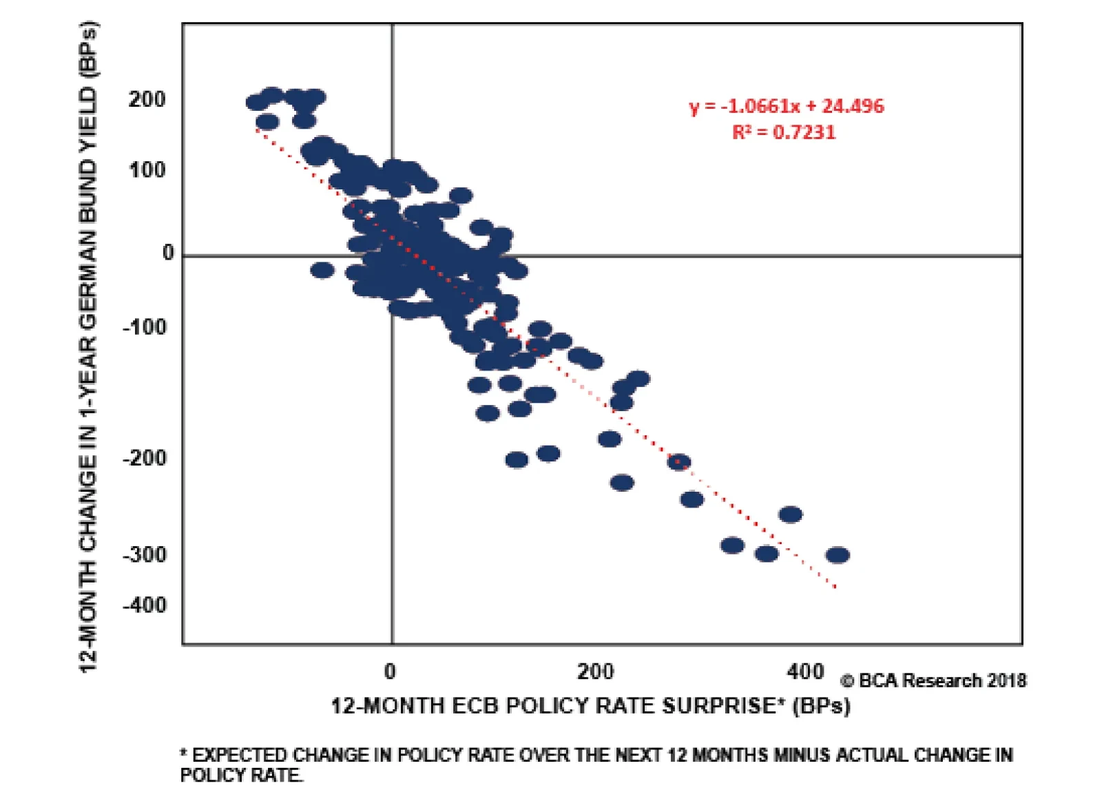
The strong correlation demonstrated between the 12-month policy rate surprises and the 12-month change in the average yield from the government bond indexes allows us to translate our "assumed" policy rate surprise over the next 12 months into expected…
Highlights The Global Golden Rule (GGR): The gap between market expectations of global central bank policy rates and realized interest rate outcomes is a reliable predictor of government bond returns. Thus, "getting the policymaker call right" is the key to outperformance for bond investors. Implied Government Bond Yields: Given the strong correlation between policy rate surprises and government bond yield changes, we can use the GGR to forecast yields one year from now based on our own assumptions of how many rate hikes (cuts) will be delivered versus what is discounted in money market yield curves. Total Return Forecasts: We can use implied government bond yield changes from the GGR to generate expected 12-month total returns for government bond indexes of different maturities, taking into account different rate hike assumptions for various central banks. Feature Chart 1Global Monetary Divergences?
Global Monetary Divergences?
Global Monetary Divergences?
This month marked the ten-year anniversary of the 2008 Lehman Brothers default, which set off a worldwide financial crisis and a massive easing of global monetary policy. Extraordinary measures - zero (or negative) interest rates, large-scale asset purchases and dovish forward guidance from policymakers - were all successful in suppressing both global bond yields and volatility over time, helping the global economy slowly heal from the crisis. Now, a decade later, such hyper-easy monetary policies are no longer required given low unemployment rates and rising inflation in the major developed economies. That can be seen today with the Federal Reserve shifting to "quantitative tightening" (letting bonds run off its swollen balance sheet) alongside steady rate hikes, the European Central Bank (ECB) set to stop net new buying of euro area bonds at year-end, and the Bank of Japan (BoJ) dramatically slowing its pace of asset purchases. BCA's Central Bank Monitors, which assess the cyclical pressure on policymakers to tighten or ease monetary policy, have collectively been calling for interest rate increases since the start of 2017. Yet our Central Bank Monetary Barometer, which measures the percentage of central banks that have tightened policy over the previous three months, shows that only 1 in 5 banks have actually delivered rate hikes of late (Chart 1). Thus, the risks are tilted towards more countries moving away from highly accommodative monetary conditions given tightening labor markets and rising inflation pressures. This now-global shift towards policy normalization has major implications for global bond investing. The focus is now returning back to more traditional drivers of government bond returns, like changes in central bank policy rates. We recently shared a Special Report published by our colleagues at our sister BCA service, U.S. Bond Strategy, describing a methodology they dubbed "The Golden Rule of Bond Investing".1 That report introduced a numerical framework that translates actual changes in the U.S. fed funds rate relative to market expectations into return forecasts for U.S. Treasuries. The historical results convincingly showed that investors who "get the Fed right" by making correct bets on changes in the funds rate versus expectations were very likely to make the right call on the direction of Treasury yields. In this Special Report, we extend that Golden Rule analysis to government bonds in the other major developed markets (DM). Our conclusion is that utilizing a "Global Golden Rule" (GGR) framework that links bond returns to unexpected changes in policy rates can help bond investors correctly forecast changes in non-U.S. bond yields. The report is set up in two sections. First, we illustrate how the GGR works and how it empirically tends to generally succeed over time for different DM bond markets. In the second section, we make use of the GGR to generate expected return forecasts for non-U.S. government bonds for a variety of interest rate "surprise" scenarios. ECB Policy Rate Surprises Dovish surprises from the ECB do reliably coincide with positive German government bond excess returns versus cash (Chart 2A). Chart 2AECB Policy Rate Surprise & Yields I
ECB Policy Rate Surprise & Yields I
ECB Policy Rate Surprise & Yields I
Chart 2BECB Policy Rate Surprise & Yields II
ECB Policy Rate Surprise & Yields II
ECB Policy Rate Surprise & Yields II
The 12-month ECB policy rate surprise and the 12-month change in the Bloomberg Barclays German Treasury index yield displays a strong positive correlation (Chart 2B). The excess returns during periods of dovish surprises is 14.4% on average and are positive 85% of the time. Hawkish surprises on the other hand, coincide with negative average excess returns of -1.5% (Chart 2C). In terms of total return, the picture is roughly the same except that under hawkish surprises, the average total return you would expect is now positive, given that it factors in coupon income (Chart 2D). Chart 2CGermany: Government Bond Index Excess Return & ECB Policy Rate Surprises (2004 - Present)
The Global Golden Rule Of Bond Investing
The Global Golden Rule Of Bond Investing
Chart 2DGermany: Government Bond Index Total Return & ECB Policy Rate Surprises (2004 - Present)
The Global Golden Rule Of Bond Investing
The Global Golden Rule Of Bond Investing
Table 1Germany: 12-Month Government Bond Index Returns And Rate Surprises (2004 - Present)
The Global Golden Rule Of Bond Investing
The Global Golden Rule Of Bond Investing
Looking ahead, the ECB should not deviate from its current dovish forward guidance of no interest rate hikes until at least the third quarter of 2019. That is somewhat consistent with the reading of the ECB monitor being almost equal to zero. Bank Of England (BoE) Policy Rate Surprises The GGR works well for the U.K. as can be seen in Chart 3A. Chart 3ABoE Policy Rate Surprise & Yields I
BoE Policy Rate Surprise & Yields I
BoE Policy Rate Surprise & Yields I
Chart 3BBoE Policy Rate Surprise & Yields II
BoE Policy Rate Surprise & Yields II
BoE Policy Rate Surprise & Yields II
The 12-month BoE policy rate surprise and the 12-month change in the Bloomberg Barclays U.K. Treasury index yield displays a strong positive correlation except for a major divergence in 1997-1998 (Chart 3B). Dovish surprises coincide with positive excess returns over cash 78% of the time and are on average equal to 6.2% over the full sample (Chart 3C and Chart 3D). As you would expect if the GGR applies, hawkish surprises coincide with negative excess returns. Chart 3CU.K.: Government Bond Index Excess Return & BoE Policy Rate Surprises (1993 - Present)
The Global Golden Rule Of Bond Investing
The Global Golden Rule Of Bond Investing
Chart 3DU.K.: Government Bond Index Total Return & BoE Policy Rate Surprises (1993 - Present)
The Global Golden Rule Of Bond Investing
The Global Golden Rule Of Bond Investing
Table 2U.K.: 12-Month Government Bond Index Returns And Rate Surprises (1993 - Present)
The Global Golden Rule Of Bond Investing
The Global Golden Rule Of Bond Investing
Looking ahead, outcomes will be biased toward dovish surprises over the next six months given the uncertain outcome of the U.K.-E.U. Brexit negotiations. Against that backdrop, the BoE will remain accommodative despite inflationary pressures building up. Bank Of Japan (BoJ) Policy Rate Surprises The GGR does not seem to work when it comes to the Japanese bond market. This reflects the fact that both the markets and the Bank of Japan (BoJ) have understood that chronic low inflation has required no changes in BoJ policy rates (Chart 4A, second panel). Chart 4ABoJ Policy Rate Surprise & Yields I
BoJ Policy Rate Surprise & Yields I
BoJ Policy Rate Surprise & Yields I
Chart 4BBoJ Policy Rate Surprise & Yields II
BoJ Policy Rate Surprise & Yields II
BoJ Policy Rate Surprise & Yields II
While the 12-month BoJ policy rate surprise and the 12-month change in the Bloomberg Barclays Japan Treasury index yield displayed a strong positive correlation pre-1998, the correlation has broken down since then (Chart 4B). Negative excess returns over cash both coincide with dovish and hawkish surprises, on average over time. Further, dovish surprises coincide with positive excess returns only 45% of the time (Chart 4C and Chart 4D). Chart 4CJapan: Government Bond Index Excess Return & BoJ Policy Rate Surprises (1994 - Present)
The Global Golden Rule Of Bond Investing
The Global Golden Rule Of Bond Investing
Chart 4DJapan: Government Bond Index Total Return & BoJ Policy Rate Surprises (1994 - Present)
The Global Golden Rule Of Bond Investing
The Global Golden Rule Of Bond Investing
Table 3Japan: 12-Month Government Bond Index Returns And Rate Surprises (1994 - Present)
The Global Golden Rule Of Bond Investing
The Global Golden Rule Of Bond Investing
Looking ahead, given that the BoJ will in all likelihood maintain its ultra-accommodative monetary policy stance in the near future, we do not expect the GGR to become more effective when applied to the Japanese bond market. Bank Of Canada (BoC) Policy Rate Surprises The GGR works relatively well for the Canadian bond market (Chart 5A). Chart 5ABoC Policy Rate Surprise & Yields I
BoC Policy Rate Surprise & Yields I
BoC Policy Rate Surprise & Yields I
Chart 5BBoC Policy Rate Surprise & Yields II
BoC Policy Rate Surprise & Yields II
BoC Policy Rate Surprise & Yields II
We observe a tight correlation between 12-month BoC policy rate surprises and the 12-month change in the Bloomberg Barclays Canada Treasury index yield, especially post-2010 (Chart 5B). Dovish surprises coincide with positive excess returns 81% of the time and 94% of the time if we look at total returns (Chart 5C and Chart 5D). Chart 5CCanada: Government Bond Index Excess Return & BoC Policy Rate Surprises (1993 - Present)
The Global Golden Rule Of Bond Investing
The Global Golden Rule Of Bond Investing
Chart 5DCanada: Government Bond Index Total Return & BoC Policy Rate Surprises (1993 - Present)
The Global Golden Rule Of Bond Investing
The Global Golden Rule Of Bond Investing
Table 4Canada: 12-Month Government Bond Index Returns And Rate Surprises (1993 - Present)
The Global Golden Rule Of Bond Investing
The Global Golden Rule Of Bond Investing
Looking ahead, the BoC will most likely continue to follow the tightening path of the Federal Reserve, admittedly with a lag. However, accelerating inflation at a time when there is no spare capacity in the Canadian economy suggests that the BoC could deliver more rate hikes than are already priced for the next 12 months. As shown in Table 4, hawkish surprises from the BoC do coincide with negative monthly excess returns of -2.8%. Reserve Bank Of Australia (RBA) Policy Rate Surprises The GGR applies extremely well to the Australian bond market (Chart 6A). Chart 6ARBA Policy Rate Surprise & Yields I
RBA Policy Rate Surprise & Yields I
RBA Policy Rate Surprise & Yields I
Chart 6BRBA Policy Rate Surprise & Yields II
RBA Policy Rate Surprise & Yields II
RBA Policy Rate Surprise & Yields II
The 12-month RBA policy rate surprise and the 12-month change in the Bloomberg Barclays Australia Treasury index yield displays the tightest correlation out of all the countries covered (Chart 6B). Dovish surprises coincide with positive excess returns 83% of the time and 96% of the time if we look at total returns (Chart 6C and Chart 6D). Turning to hawkish surprises, they reliably coincide with negative excess returns. Chart 6CAustralia: Government Bond Index Excess Return & RBA Policy Rate Surprises (1994 - Present)
The Global Golden Rule Of Bond Investing
The Global Golden Rule Of Bond Investing
Chart 6DAustralia: Government Bond Index Total Return & RBA Policy Rate Surprises (1994 - Present)
The Global Golden Rule Of Bond Investing
The Global Golden Rule Of Bond Investing
Table 5Australia: 12-Month Government Bond Index Returns And Rate Surprises (1994 - Present)
The Global Golden Rule Of Bond Investing
The Global Golden Rule Of Bond Investing
As can be seen on the bottom panel of Chart 6A, the RBA Monitor has been rapidly falling since 2016 and now stands in the "easier monetary policy" required. However, the RBA will likely have to see a rise in unemployment or a decline in realized inflation before it considers cutting rates, which raises a risk of "hawkish" surprises if the market begins to price in rate cuts. Reserve Bank Of New Zealand (RBNZ) Policy Rate Surprises The GGR works fairly well for Nez Zealand (NZ) government bonds (Chart 7A). Chart 7ARBNZ Policy Rate Surprise & Yields I
RBNZ Policy Rate Surprise & Yields I
RBNZ Policy Rate Surprise & Yields I
Chart 7BRBNZ Policy Rate Surprise & Yields II
RBNZ Policy Rate Surprise & Yields II
RBNZ Policy Rate Surprise & Yields II
12-month RBNZ policy rate surprises and the 12-month change in the Bloomberg Barclays NZ Treasury yield exhibit a decent correlation (Chart 7B). Unusually, NZ is the only bond market covered in this report where both dovish and hawkish surprises coincide with positive excess returns on average, although positive episodes are much less frequent for hawkish surprises than for dovish surprises; respectively 55% and 86% (Chart 7C and Chart 7D). Chart 7CNZ: Government Bond Index Excess Return & RBNZ Policy Rate Surprises (2000 - Present)
The Global Golden Rule Of Bond Investing
The Global Golden Rule Of Bond Investing
Chart 7DNZ: Government Bond Index Total Return & RBNZ Policy Rate Surprises (2000 - Present)
The Global Golden Rule Of Bond Investing
The Global Golden Rule Of Bond Investing
Table 6New Zealand: 12-Month Government Bond Index Returns And Rate Surprises (2000 - Present)
The Global Golden Rule Of Bond Investing
The Global Golden Rule Of Bond Investing
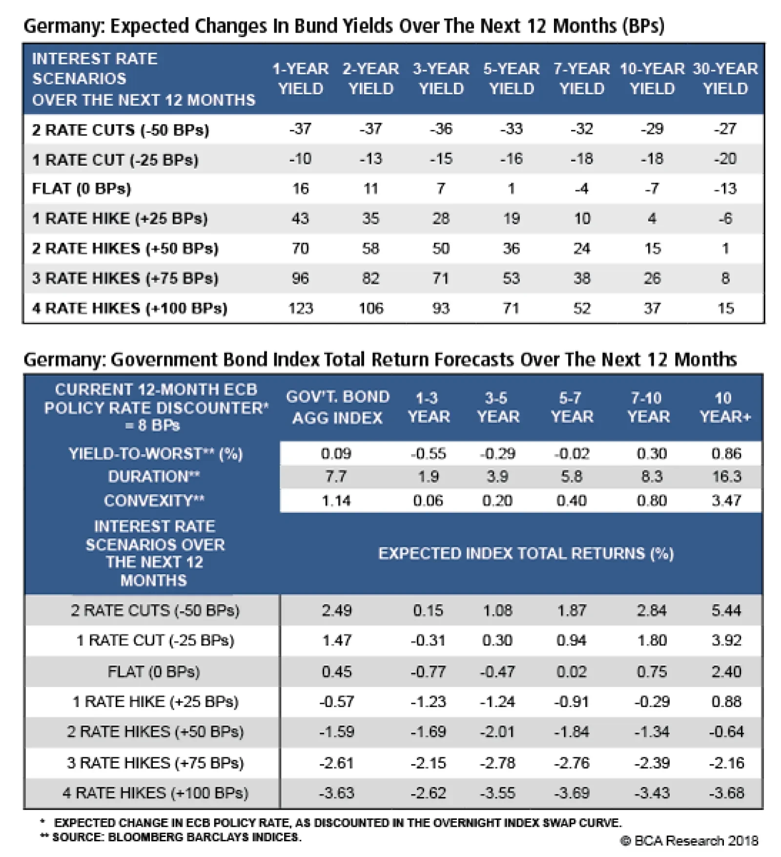
Looking ahead, the RBNZ has already provided forward guidance indicating that the Overnight Cash Rate (OCR) will most likely stay flat until 2020 - an assessment that we agree with, so the odds are against any policy surprises over at least the next 6-12 months. Using The Global Golden Rule To Forecast Government Bond Returns The practical application of the GGR is that it can be used as a framework for generating expected changes in yields and calculating total return forecasts for global government bond indices. The strong correlation demonstrated in the previous section between the 12-month policy rate surprises and the 12-month change in the average yield from the government bond indexes allows us to translate our "assumed" policy rate surprise over the next 12 months into expected changes in yields along the curve. With these expected yield changes, we can simply generate expected total returns using the following formula: Expected Total Return = Yield - (Duration*Expected Change In Yield) + 0.5*Convexity*E(DY2) E(DY2) = 1-year trailing estimate of yield volatility It is important to note that we would not give too much importance to what this analysis yields for longer-dated bonds. As shown in the Appendices, once we move into longer government bond maturities, the correlation between the policy rate surprise and the change in yields declines or even becomes non-existent for some countries. This result should not be surprising, as longer-term yields are driven by other factors besides simply changes in interest rate expectations. Inflation expectations, government debt levels and demand from longer-term investors like pension funds all can have a more outsized influence on the path of longer-term bond yields relative to the shorter-end. That results in much more uncertainty when it comes to the total return forecasts for long-dated maturities calculated with this framework. Practically speaking, we are not encouraging our readers to blindly follow that yield and return expectations generated by the GGR, even for bond markets where it clearly seems to be working over time. Rather, the GGR can be integrated in a larger asset-allocation framework for a global fixed-income portfolio by providing one possible set of bond market outcomes. On a total return basis, the results presented below, interpreted alongside the readings on the BCA Central Bank monitors, suggest that investors should be underweight core Euro Area (Germany, France and Italy), Australia and New Zealand while remaining overweight the U.K. and Canada over the next twelve months. As for Japan, given the likelihood that BoJ will leave its policy rate flat, the results hint at a neutral allocation. Jeremie Peloso, Research Analyst jeremie@bcaresearch.com Robert Robis, CFA, Senior Vice President Global Fixed Income Strategy rrobis@bcaresearch.com 1 Please see U.S. Bond Strategy Special Report, "The Golden Rule Of Bond Investing", dated July 24, 2018, available at usbs.bcaresearch.com. 2 Please see Global Fixed Income Strategy Weekly Report, "BCA Central Bank Monitor Chartbook: Divergences Opening Up," dated September 19, 2018, available at gfis.bcaresearch.com. Global Golden Rule: Germany In light of the forward guidance ECB President Mario Draghi has been providing to the markets, it appears that the most likely scenario over the next 12 months is for the ECB to keep interest rates on hold. Based on the strong relationships between 12-month ECB policy rate surprises and 12-month changes in yields along the curve (Appendix A), a flat interest rate scenario would be bond bearish for German government bonds especially at the short end of the curve with the 1-year German yield expected to rise by 16bps (Table 7A). Table 7AGermany: Expected Changes In Bund Yields Over The Next 12 Months (BPs)
The Global Golden Rule Of Bond Investing
The Global Golden Rule Of Bond Investing
Using the expected change in yields thus inferred by the policy rate surprise, the German government bond aggregate index is forecasted to return 0.45% over the next 12 months (Table 7B). Table 7BGermany: Government Bond Index Total Return Forecasts Over The Next 12 Months
The Global Golden Rule Of Bond Investing
The Global Golden Rule Of Bond Investing
Global Golden Rule: U.K. Markets are currently discounting only 21bps of rate hikes in the U.K. over the next year. Thus, even a scenario where the BoE delivers only a single 25bp rate hike would be bearish for U.K. Gilts, especially at the short-end of the curve. Applying the GGR, 1- and 3-year Gilt yields would be expected to rise by 20bps and 10bps respectively (Table 8A). Table 8AU.K.: Expected Changes In Gilt Yields Over The Next 12 Months (BPs)
The Global Golden Rule Of Bond Investing
The Global Golden Rule Of Bond Investing
Interpolating these expected yield changes, the 1-3 year government bond index total return forecast would be 0.46%. On the other hand, if the BoE prefers to keep rates on hold given the uncertainty of the Brexit outcome, that same 1-3 year government bond index is forecasted to deliver 0.97% of total return over the next 12 months (Table 9B). This is our current base case scenario for Gilts. Table 8BU.K.: Government Bond Index Total Return Forecasts Over The Next 12 Months
The Global Golden Rule Of Bond Investing
The Global Golden Rule Of Bond Investing
Global Golden Rule: Japan Despite many rumors to the contrary earlier this year, the base case view remains that the BoJ will not change its stance on monetary policy anytime soon. As such, the expected changes in JGB yields under a flat interest rate scenario over the next 12 months are close to zero at the short end of the curve and rather bond bullish at the longer end of the curve; for instance, the 30-year JGB yield would be expected to rally by 9bps (Table 9A). Table 9AJapan: Expected Changes In JGB Yields Over The Next 12 Months (BPs)
The Global Golden Rule Of Bond Investing
The Global Golden Rule Of Bond Investing
In that most likely scenario, the Japanese government bond index is forecasted to deliver 0.83% of total return over the next 12 months. In the event that the BoJ surprises the markets by delivering one rate hike of 25bps, it would be bond bearish for JGBs and the total return forecasts for the government bond indices would be negative, regardless of the maturity (Table 9B). Table 9BJapan: Government Bond Index Total Return Forecasts Over The Next 12 Months
The Global Golden Rule Of Bond Investing
The Global Golden Rule Of Bond Investing
Global Golden Rule: Canada Will the Bank of Canada follow the footsteps of the Fed? The markets certainly seem to think so, with more than three 25bps rate hikes priced in for next 12 months in the OIS curve. Table 10ACanada: Expected Changes In Government Bond Yields Over The Next 12 Months (BPs)
The Global Golden Rule Of Bond Investing
The Global Golden Rule Of Bond Investing
That scenario would be outright bearish for Canadian government bonds, with 1- and 2-year yields rising by 16bps and 21bps, respectively (Table 10A). In terms of total returns, the GGR framework forecasts that with 75bps of rate hikes, the Canadian government bond aggregate index would deliver a positive return of 2.35% (Table 10B). This is because 75bps of hikes are currently discounted in the Canadian OIS curve, thus it would neither be a hawkish nor dovish surprise. Table 10BCanada: Government Bond Index Total Return Forecasts Over The Next 12 Months
The Global Golden Rule Of Bond Investing
The Global Golden Rule Of Bond Investing
Global Golden Rule: Australia The RBA Monitor just dipped below the zero line, implying that easier monetary policy is required based on financial and economic data. Table 11A shows that a rate cut delivered by the RBA in the next 12 months would be bond bullish for Aussie yields, especially at the long end of the curve, where the 30-year Aussie bond yield would fall by 34bps. Table 11AAustralia: Expected Changes In Aussie Yields Over The Next 12 Months (BPs)
The Global Golden Rule Of Bond Investing
The Global Golden Rule Of Bond Investing
Of all the interest rate scenarios presented in Table 11B, the two rate cut scenarios would return the highest total returns. For instance, the Australian government bond aggregate index would return 2.80% and 3.90% in the event of one and two 25bps rate hikes, respectively. Table 11BAustralia: Government Bond Index Total Return Forecasts Over The Next 12 Months
The Global Golden Rule Of Bond Investing
The Global Golden Rule Of Bond Investing
Global Golden Rule: New Zealand Our view is that the Reserve Bank of New Zealand will stay on hold for a while longer, which is broadly the same message conveyed by the RBNZ Monitor being positive, but very close to 0. With that in mind, a flat interest rate scenario appears to be bond bearish for the NZ bond yields, except for the longer end of the curve (Table 12A). Table 12ANew Zealand: Expected Changes In NZ Yields Over The Next 12 Months (BPs)
The Global Golden Rule Of Bond Investing
The Global Golden Rule Of Bond Investing
Table 12BNew Zealand: Government Bond Index Total
The Global Golden Rule Of Bond Investing
The Global Golden Rule Of Bond Investing
For New Zealand, the government bond aggregate bond index is the only index provided by Bloomberg Barclays, as opposed to the other countries in our analysis where different maturities are given. In the flat interest rate scenario, the total return forecast for the overall index would be of 2.53% over the next 12 months. Appendix A: Germany Chart 1Change In 1-Year German Bund Yield##BR##Vs. 12-Month ECB Policy Rate Surprise
The Global Golden Rule Of Bond Investing
The Global Golden Rule Of Bond Investing
Chart 2Change In 2-Year German Bund Yield##BR##Vs. 12-Month ECB Policy Rate Surprise
The Global Golden Rule Of Bond Investing
The Global Golden Rule Of Bond Investing
Chart 3Change In 3-Year German Bund Yield##BR##Vs. 12-Month ECB Policy Rate Surprise
The Global Golden Rule Of Bond Investing
The Global Golden Rule Of Bond Investing
Chart 4Change In 5-Year German Bund Yield##BR##Vs. 12-Month ECB Policy Rate Surprise
The Global Golden Rule Of Bond Investing
The Global Golden Rule Of Bond Investing
Chart 5Change In 7-Year German Bund Yield##BR##Vs. 12-Month ECB Policy Rate Surprise
The Global Golden Rule Of Bond Investing
The Global Golden Rule Of Bond Investing
Chart 6Change In 10-Year German Bund Yield##BR##Vs. 12-Month ECB Policy Rate Surprise
The Global Golden Rule Of Bond Investing
The Global Golden Rule Of Bond Investing
Chart 7Change In 30-Year German Bund Yield##BR##Vs. 12-Month ECB Policy Rate Surprise
The Global Golden Rule Of Bond Investing
The Global Golden Rule Of Bond Investing
Appendix B: France Chart 8Change In 1-Year French OAT Yield##BR##Vs. 12-Month ECB Policy Rate Surprise
The Global Golden Rule Of Bond Investing
The Global Golden Rule Of Bond Investing
Chart 9Change In 2-Year French OAT Yield##BR##Vs. 12-Month ECB Policy Rate Surprise
The Global Golden Rule Of Bond Investing
The Global Golden Rule Of Bond Investing
Chart 10Change In 3-Year French OAT Yield##BR##Vs. 12-Month ECB Policy Rate Surprise
The Global Golden Rule Of Bond Investing
The Global Golden Rule Of Bond Investing
Chart 11Change In 5-Year French OAT Yield##BR##Vs. 12-Month ECB Policy Rate Surprise
The Global Golden Rule Of Bond Investing
The Global Golden Rule Of Bond Investing
Chart 12Change In 7-Year French OAT Yield##BR##Vs. 12-Month ECB Policy Rate Surprise
The Global Golden Rule Of Bond Investing
The Global Golden Rule Of Bond Investing
Chart 13Change In 10-Year French OAT Yield##BR##Vs. 12-Month ECB Policy Rate Surprise
The Global Golden Rule Of Bond Investing
The Global Golden Rule Of Bond Investing
Chart 14Change In 30-Year French OAT Yield##BR##Vs. 12-Month ECB Policy Rate Surprise
The Global Golden Rule Of Bond Investing
The Global Golden Rule Of Bond Investing
Appendix C: Italy Chart 15Change In 1-Year Italian Gov't Bond Yield##BR##Vs. 12-Month ECB Policy Rate Surprise
The Global Golden Rule Of Bond Investing
The Global Golden Rule Of Bond Investing
Chart 16Change In 2-Year Italian Gov't Bond Yield##BR##Vs. 12-Month ECB Policy Rate Surprise
The Global Golden Rule Of Bond Investing
The Global Golden Rule Of Bond Investing
Chart 17Change In 3-Year Italian Gov't Bond Yield##BR##Vs. 12-Month ECB Policy Rate Surprise
The Global Golden Rule Of Bond Investing
The Global Golden Rule Of Bond Investing
Chart 18Change In 5-Year Italian Gov't Bond Yield##BR##Vs. 12-Month ECB Policy Rate Surprise
The Global Golden Rule Of Bond Investing
The Global Golden Rule Of Bond Investing
Chart 19Change In 7-Year Italian Gov't Bond Yield##BR##Vs. 12-Month ECB Policy Rate Surprise
The Global Golden Rule Of Bond Investing
The Global Golden Rule Of Bond Investing
Chart 20Change In 10-Year Italian Gov't Bond Yield##BR##Vs. 12-Month ECB Policy Rate Surprise
The Global Golden Rule Of Bond Investing
The Global Golden Rule Of Bond Investing
Chart 21Change In 30-Year Italian Gov't Bond Yield##BR##Vs. 12-Month ECB Policy Rate Surprise
The Global Golden Rule Of Bond Investing
The Global Golden Rule Of Bond Investing
Appendix D: U.K. Chart 22Change In 1-Year Gilts Yield##BR##Vs. 12-Month BoE Policy Rate Surprise
The Global Golden Rule Of Bond Investing
The Global Golden Rule Of Bond Investing
Chart 23Change In 2-Year Gilts Yield##BR##Vs. 12-Month BoE Policy Rate Surprise
The Global Golden Rule Of Bond Investing
The Global Golden Rule Of Bond Investing
Chart 24Change In 3-Year Gilts Yield##BR##Vs. 12-Month BoE Policy Rate Surprise
The Global Golden Rule Of Bond Investing
The Global Golden Rule Of Bond Investing
Chart 25Change In 5-Year Gilts Yield##BR##Vs. 12-Month BoE Policy Rate Surprise
The Global Golden Rule Of Bond Investing
The Global Golden Rule Of Bond Investing
Chart 26Change In 7-Year Gilts Yield##BR##Vs. 12-Month BoE Policy Rate Surprise
The Global Golden Rule Of Bond Investing
The Global Golden Rule Of Bond Investing
Chart 27Change In 10-Year Gilts Yield##BR##Vs. 12-Month BoE Policy Rate Surprise
The Global Golden Rule Of Bond Investing
The Global Golden Rule Of Bond Investing
Chart 28Change In 30-Year Gilts Yield##BR##Vs. 12-Month BoE Policy Rate Surprise
The Global Golden Rule Of Bond Investing
The Global Golden Rule Of Bond Investing
Appendix E: Japan Chart 29Change In 1-Year Japanese JGB Yield##BR##Vs. 12-Month BoJ Policy Rate Surprise
The Global Golden Rule Of Bond Investing
The Global Golden Rule Of Bond Investing
Chart 30Change In 2-Year Japanese JGB Yield##BR##Vs. 12-Month BoJ Policy Rate Surprise
The Global Golden Rule Of Bond Investing
The Global Golden Rule Of Bond Investing
Chart 31Change In 3-Year Japanese JGB Yield##BR##Vs. 12-Month BoJ Policy Rate Surprise
The Global Golden Rule Of Bond Investing
The Global Golden Rule Of Bond Investing
Chart 32Change In 5-Year Japanese JGB Yield##BR##Vs. 12-Month BoJ Policy Rate Surprise
The Global Golden Rule Of Bond Investing
The Global Golden Rule Of Bond Investing
Chart 33Change In 7-Year Japanese JGB Yield##BR##Vs. 12-Month BoJ Policy Rate Surprise
The Global Golden Rule Of Bond Investing
The Global Golden Rule Of Bond Investing
Chart 34Change In 10-Year Japanese JGB Yield##BR##Vs. 12-Month BoJ Policy Rate Surprise
The Global Golden Rule Of Bond Investing
The Global Golden Rule Of Bond Investing
Chart 35Change In 30-Year Japanese JGB Yield##BR##Vs. 12-Month BoJ Policy Rate Surprise
The Global Golden Rule Of Bond Investing
The Global Golden Rule Of Bond Investing
Appendix F: Canada Chart 36Change In 1-Year Canadian Yield##BR##Vs. 12-Month BoC Policy Rate Surprise
The Global Golden Rule Of Bond Investing
The Global Golden Rule Of Bond Investing
Chart 37Change In 2-Year Canadian Yield##BR##Vs. 12-Month BoC Policy Rate Surprise
The Global Golden Rule Of Bond Investing
The Global Golden Rule Of Bond Investing
Chart 38Change In 3-Year Canadian Yield##BR##Vs. 12-Month BoC Policy Rate Surprise
The Global Golden Rule Of Bond Investing
The Global Golden Rule Of Bond Investing
Chart 39Change In 5-Year Canadian Yield##BR##Vs. 12-Month BoC Policy Rate Surprise
The Global Golden Rule Of Bond Investing
The Global Golden Rule Of Bond Investing
Chart 40Change In 7-Year Canadian Yield##BR##Vs. 12-Month BoC Policy Rate Surprise
The Global Golden Rule Of Bond Investing
The Global Golden Rule Of Bond Investing
Chart 41Change In 10-Year Canadian Yield##BR##Vs. 12-Month BoC Policy Rate Surprise
The Global Golden Rule Of Bond Investing
The Global Golden Rule Of Bond Investing
Chart 42Change In 30-Year Canadian Yield##BR##Vs. 12-Month BoC Policy Rate Surprise
The Global Golden Rule Of Bond Investing
The Global Golden Rule Of Bond Investing
Appendix G: Australia Chart 43Change In 1-Year Aussie Yield##BR##Vs. 12-Month RBA Policy Rate Surprise
The Global Golden Rule Of Bond Investing
The Global Golden Rule Of Bond Investing
Chart 44Change In 2-Year Aussie Yield##BR##Vs. 12-Month RBA Policy Rate Surprise
The Global Golden Rule Of Bond Investing
The Global Golden Rule Of Bond Investing
Chart 45Change In 3-Year Aussie Yield##BR##Vs. 12-Month RBA Policy Rate Surprise
The Global Golden Rule Of Bond Investing
The Global Golden Rule Of Bond Investing
Chart 46Change In 5-Year Aussie Yield##BR##Vs. 12-Month RBA Policy Rate Surprise
The Global Golden Rule Of Bond Investing
The Global Golden Rule Of Bond Investing
Chart 47Change In 7-Year Aussie Yield##BR##Vs. 12-Month RBA Policy Rate Surprise
The Global Golden Rule Of Bond Investing
The Global Golden Rule Of Bond Investing
Chart 48Change In 10-Year Aussie Yield##BR##Vs. 12-Month RBA Policy Rate Surprise
The Global Golden Rule Of Bond Investing
The Global Golden Rule Of Bond Investing
Appendix H: New Zealand Chart 49Change In 1-Year NZ Yield##BR##Vs. 12-Month RBNZ Policy Rate Surprise
The Global Golden Rule Of Bond Investing
The Global Golden Rule Of Bond Investing
Chart 50Change In 2-Year NZ Yield##BR##Vs. 12-Month RBNZ Policy Rate Surprise
The Global Golden Rule Of Bond Investing
The Global Golden Rule Of Bond Investing
Chart 51Change In 3-Year NZ Yield##BR##Vs. 12-Month RBNZ Policy Rate Surprise
The Global Golden Rule Of Bond Investing
The Global Golden Rule Of Bond Investing
Chart 52Change In 5-Year NZ Yield##BR##Vs. 12-Month RBNZ Policy Rate Surprise
The Global Golden Rule Of Bond Investing
The Global Golden Rule Of Bond Investing
Chart 53Change In 7-Year NZ Yield##BR##Vs. 12-Month RBNZ Policy Rate Surprise
The Global Golden Rule Of Bond Investing
The Global Golden Rule Of Bond Investing
Chart 54Change In 10-Year NZ Yield##BR##Vs. 12-Month RBNZ Policy Rate Surprise
The Global Golden Rule Of Bond Investing
The Global Golden Rule Of Bond Investing
Our Global Investment Strategy team recommended this position past June as a means to benefit from potential China downside, and U.S. upside. A weaker yuan and Chinese economy will raise raw material costs to Chinese firms. This will hurt commodity prices.…
There are three significant data releases for the euro area next week: the IFO Business Climate Index on Monday, the European Commission’s economic confidence indicator on Thursday, and consumer prices on Friday. Consensus expectations for the IFO call for a…
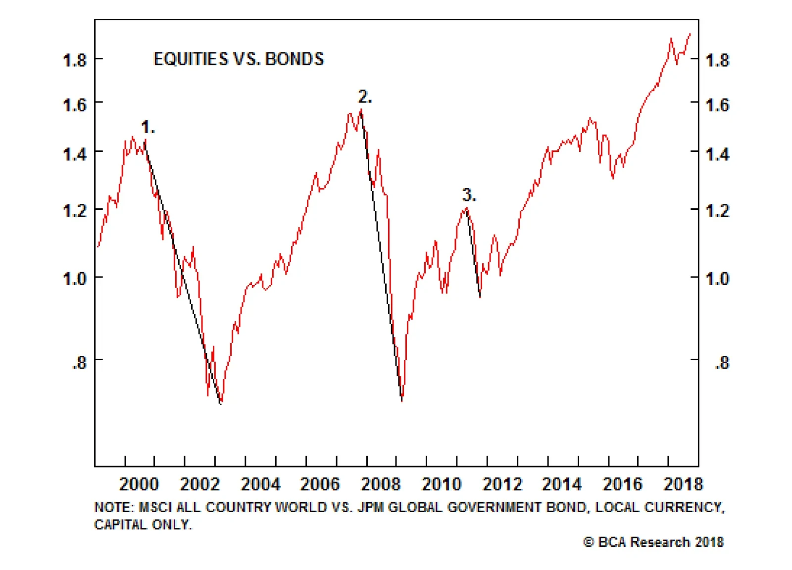
There have been three major financial market downturns, defined as a greater-than-six-month period when equities underperform bonds by more than 20 percent, in the 21th century (see chart). The twenty-first century’s major economic downturns have all…
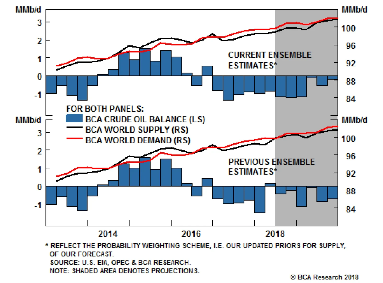
Since 2017, the factor model used by our commodity strategists to forecast oil prices shows that brent prices have been supported by two drivers that are simultaneously pushing price estimates higher: First, strong compliance of OPEC 2.0 members to the…
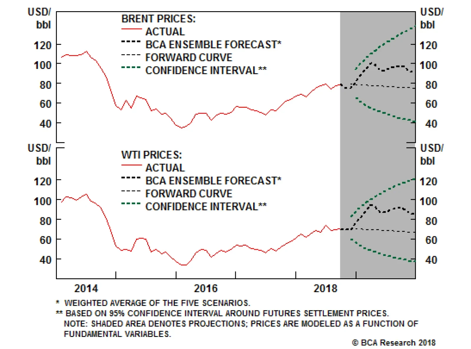
With the loss of Iranian exports occurring faster and sooner than expected, and Venezuela remaining on the brink of collapse, senior energy officials from the U.S., Russia, Saudi Arabia are going to great lengths to reassure their domestic consumers…
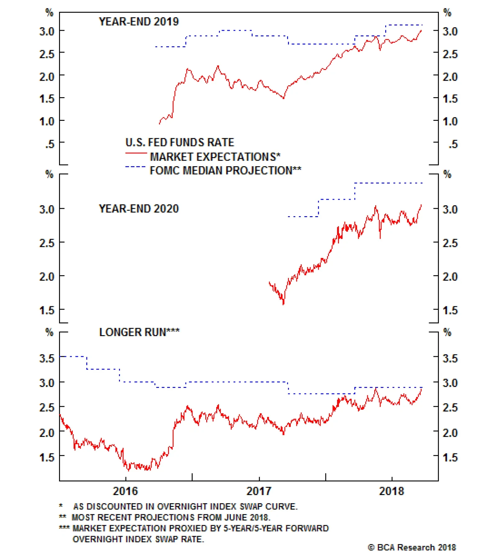
Highlights We review last year's "Three Tantalizing Trades" and offer four additional ones: Trade #1: Long June 2019 Fed funds futures contract/short Dec 2020 Fed funds futures contract Trade #2: Long USD/CNY Trade #3: Short AUD/CAD Trade #4: Long EM stocks with near-term downside put protection Feature A Review Of Last Year's "Three Tantalizing Trades" I had the pleasure of speaking at BCA's last Annual Investment Conference on September 25th, 2017, where I presented the following three trade ideas (Chart 1): 1. Short December 2018 Fed funds futures We closed this trade for a profit of 70 basis points. Had we held on, it would be up 92 basis points as of the time of this writing. 2. Long global industrial equities/short utilities We closed this trade on February 1st for a gain of 12%, as downside risks to global growth began to mount. This proved to be a timely decision, as the trade would be up only 6.1% had we kept it on. We would not re-enter this trade at present. 3. Short 20-year JGBs/long 5-year JGBs This trade struggled for much of 2018 but sprung back to life in August. It is up 0.6% since we initiated it. We still like the trade over the long haul. Investors are grossly underestimating the risk that Japanese inflation will move materially higher as an aging population creates a shortage of workers and a concomitant decline in the national savings rate. We also think the government will try to egg on any acceleration in consumer prices in order to inflate away its debt burden. In the near term, however, the trade could struggle if a combination of weaker EM growth and an increase in the value of the trade-weighted yen cause inflation expectations to decline. Four Additional Trades Trade #1: Long June 2019 Fed funds futures contract/short December 2020 Fed funds futures contract Investors expect U.S. short-term rates to rise to 2.38% by the end of 2018 and 2.85% by the end of 2019. The 47 basis points in tightening priced in for next year is less than the 75 basis points in hikes implied by the Fed dots. Investors appear to have bought into Larry Summers' secular stagnation thesis. They are convinced that short rates will not be able to rise above 3% without triggering a recession (Chart 2). Chart 1Revisiting Last Year's Three Tantalizing Trades
Revisiting Last Year's Three Tantalizing Trades
Revisiting Last Year's Three Tantalizing Trades
Chart 2Markets Expect No Fed Hikes Beyond Next Year
Four Tantalizing Trades
Four Tantalizing Trades
Regardless of what one thinks of Summers' thesis, it must be acknowledged that it is a theory about the long-term drivers of the neutral rate of interest. Over a shorter-term cyclical horizon, many factors can influence the neutral rate. Critically, most of these factors are pushing it higher: Fiscal policy is extremely stimulative. The IMF estimates that the U.S. cyclically-adjusted budget deficit will reach 6.8% of GDP in 2019 compared to 3.6% of GDP in 2015. In contrast, the euro area is projected to run a deficit of only 0.8% of GDP next year, little changed from a deficit of 0.9% it ran in 2015 (Chart 3). The relatively more expansionary nature of U.S. fiscal policy is one key reason why the Fed can raise rates while the ECB cannot. Credit growth has picked up. After a prolonged deleveraging cycle, private-sector nonfinancial debt is rising faster than GDP (Chart 4). The recent easing in The Conference Board's Leading Credit Index suggests that this trend will continue (Chart 5). Wage growth is accelerating. Average hourly earnings surprised on the upside in August, with the year-over-year change rising to a cycle high of 2.9%. This followed a stronger reading in the Employment Cost Index in the second quarter. A simple correlation with the quits rate suggests that there is plenty of upside for wage growth (Chart 6). Faster wage growth will put more money into workers pockets who will then spend it. The savings rate has scope to fall. The personal savings rate currently stands at 6.7%, more than two percentage points higher than what one would expect based on the current ratio of household net worth-to-disposable income (Chart 7). If the savings rate were to fall by two points over the next two years, it would add 1.5% of GDP to aggregate demand. Chart 3U.S. Fiscal Policy Is More Expansionary Than The Euro Area
U.S. Fiscal Policy Is More Expansionary Than The Euro Area
U.S. Fiscal Policy Is More Expansionary Than The Euro Area
Chart 4U.S. Private-Sector Nonfinancial Debt Is Rising At Close To Its Historic Trend
U.S. Private-Sector Nonfinancial Debt Is Rising At Close To Its Historic Trend
U.S. Private-Sector Nonfinancial Debt Is Rising At Close To Its Historic Trend
Chart 5U.S. Credit Growth Will Remain Strong
U.S. Credit Growth Will Remain Strong
U.S. Credit Growth Will Remain Strong
Chart 6Quits Rate Is Signaling That There Is Upside For Wage Growth
Quits Rate Is Signaling That There Is Upside For Wage Growth
Quits Rate Is Signaling That There Is Upside For Wage Growth
Chart 7The Personal Savings Rate Has Room To Fall
Four Tantalizing Trades
Four Tantalizing Trades
A back-of-the-envelope calculation suggests that these cyclical factors will permit the Fed to raise rates to 5% by 2020, almost double what the market is discounting.1 A more hawkish-than-expected Fed will bid up the value of the greenback. A stronger dollar, in turn, will undermine emerging markets, which have seen foreign-currency debts balloon over the past six years (Chart 8). The deflationary effects of a stronger dollar and falling commodity prices could temporarily cause investors to price out some hikes over the next few quarters. With that in mind, we recommend shorting the December 2020 Fed funds futures contract, while going long the June 2019 contract. The first leg of the trade captures our expectation that the market will revise up its estimate the terminal rate, while the second leg captures near-term risks to global growth. The gap between the two contracts has widened over the past few days as we have prepared this report, but at 21 basis points, it has plenty of room to increase further (Chart 9). Chart 8EM Dollar Debt Is High
EM Dollar Debt Is High
EM Dollar Debt Is High
Chart 9U.S. Rate Expectations Are Too Low Beyond Mid-2019
U.S. Rate Expectations Are Too Low Beyond Mid-2019
U.S. Rate Expectations Are Too Low Beyond Mid-2019
Trade #2: Long USD/CNY China's economy is slowing, which has prompted the government to inject liquidity into the financial system. The spread in 1-year swap rates between the U.S. and China has fallen from about 3% earlier this year to 0.6% at present, taking the yuan down with it (Chart 10). It is doubtful that China will be willing to match - let alone exceed - U.S. rate hikes. This suggests that USD/CNY will appreciate. China's real trade-weighted exchange rate has weakened during the past four months, but is up 25% over the past decade (Chart 11). U.S. tariffs on $250 billion (and counting) of Chinese imports threaten to erode export competitiveness, making a further devaluation necessary. Chart 10USD/CNY Has Tracked China-U.S. Interest Rate Differentials
USD/CNY Has Tracked China-U.S. Interest Rate Differentials
USD/CNY Has Tracked China-U.S. Interest Rate Differentials
Chart 11The RMB Is Still Quite Strong
The RMB Is Still Quite Strong
The RMB Is Still Quite Strong
President Trump will oppose a weaker yuan. However, just as China's actions earlier this year to strengthen its currency did not prevent the U.S. from imposing tariffs, it is doubtful that efforts by the Chinese authorities to talk up the yuan would appease Trump. Besides, China needs a weaker currency. The Chinese economy produces too much and spends too little. The result is excess savings, epitomized most clearly in a national savings rate of 46%. As a matter of arithmetic, national savings need to be transformed either into domestic investment or exported abroad via a current account surplus. China has concentrated on the former strategy over the past decade. The problem is that this approach has run into diminishing returns. Chart 12 shows that the capital stock has risen dramatically as a share of GDP. As my colleague Jonathan LaBerge has documented, the rate of return on assets among Chinese state-owned companies, which have been the main driver of rising corporate leverage, has fallen below their borrowing costs (Chart 13).2 Chart 12China's Capital Stock Has Grown Alongside Rising Debt Levels
China's Capital Stock Has Grown Alongside Rising Debt Levels
China's Capital Stock Has Grown Alongside Rising Debt Levels
Chart 13China: Rate Of Return On Assets Below Borrowing Costs For State-Owned Companies
China: Rate Of Return On Assets Below Borrowing Costs For State-Owned Companies
China: Rate Of Return On Assets Below Borrowing Costs For State-Owned Companies
Now that the economy is awash in excess capacity, the authorities will need to steer more excess production abroad. This will require a larger current account surplus which, in turn, will necessitate a relatively cheap currency. The dollar is currently working off overbought technical conditions, a risk we flagged in our August 31st report.3 That process should be complete over the next few weeks. Meanwhile, hopes of a massive Chinese stimulus focused on fiscal/credit easing will fade. The combination of these two forces will push up USD/CNY above the psychologically-critical 7 handle by the end of the year. Trade #3: Short AUD/CAD A weaker yuan will raise raw material costs to Chinese firms. This will hurt commodity prices. Industrial metals are much more vulnerable to slower Chinese growth than oil. Chart 14 shows that China consumes close to half of all the copper, nickel, aluminum, zinc, and iron ore produced in the world, compared to only 15% of oil output. Our expectation that developed economy growth will hold up better than EM growth over the next few quarters implies that oil will outperform industrial metals. Oil is also supported by a tighter supply backdrop, particularly given the downside risks to Iranian and Venezuelan crude exports. A bet on oil over metals is a bet on DM over EM growth in general, and the Canadian dollar over the Australian dollar specifically (Chart 15). Canada exports more oil than metals, while Australian exports are dominated by ores and metals. In terms of valuations, the Canadian dollar is still somewhat cheap relative to the Aussie dollar based on our FX team's long-term valuation model (Chart 16). Chart 14China Is A More Dominant Consumer Of Metals Than Oil
China Is A More Dominant Consumer Of Metals Than Oil
China Is A More Dominant Consumer Of Metals Than Oil
Chart 15Oil Over Metals = CAD Over AUD
Oil Over Metals = CAD Over AUD
Oil Over Metals = CAD Over AUD
Chart 16Canadian Dollar Still Somewhat Cheap Versus The Aussie Dollar
Canadian Dollar Still Somewhat Cheap Versus The Aussie Dollar
Canadian Dollar Still Somewhat Cheap Versus The Aussie Dollar
The loonie has been weighed down by ongoing fears that Canada will be left out of a renegotiated NAFTA. However, our geopolitical strategists believe that the Trump administration is trying to focus more on China, against whom the case for unfair trade practices is far easier to make. The U.S. has already negotiated a trade deal with Mexico and an agreement with Canada is more likely than not. If a new deal is struck, the Canadian dollar will rally. We recommended going short AUD/CAD on June 28. The trade is up 3.4%, carry-adjusted, since then. Stick with it. Trade #4: Long EM stocks with near-term downside put protection It is too early to call a bottom in EM assets. Valuations have not yet reached washed-out levels (Chart 17). Bottom fishers still abound, as evidenced by the fact that the number of shares outstanding in the MSCI iShares Turkish ETF has almost tripled since early April (Chart 18). However, at some point - probably in the first half of next year - investors will liquidate their remaining bullish EM bets. During the 1990s, this capitulation point occurred shortly after the collapse of Long-Term Capital Management in September 1998. EM equities fell by 26% between April 21, 1998 and June 15, 1998. After a half-hearted attempt at a rally, EM stocks tumbled again in July, falling by 35% between July 17 and September 10. The second leg of the EM selloff brought down the S&P 500 by 22%. Thanks to a series of well-telegraphed Fed rate cuts, global markets stabilized on October 8th (Chart 19). The S&P 500 surged by 68% over the next 18 months. The MSCI EM index more than doubled in dollar terms over this period. EM stocks outperformed U.S. equities by a whopping 71% between February 1999 and February 2000. Europe also outperformed the U.S. starting in mid-1999. Value stocks, which had lagged growth stocks over the prior six years, also finally gained the upper hand. Chart 17EM Assets: Valuations Not Yet At Washed Out Levels
EM Assets: Valuations Not Yet At Washed Out Levels
EM Assets: Valuations Not Yet At Washed Out Levels
Chart 18EM Bottom Fishers Still Abound
EM Bottom Fishers Still Abound
EM Bottom Fishers Still Abound
Chart 19The ''Great Equity Rotation'' Is Coming: A Roadmap From The 1990s
The ''Great Equity Rotation'' Is Coming: A Roadmap From The 1990s
The ''Great Equity Rotation'' Is Coming: A Roadmap From The 1990s
The "Great Equity Rotation" is coming. All the trades that have suffered lately - overweight EM, long Europe/short U.S., long cyclicals/short defensives, long value/short growth - will get their day in the sun. Investors can prepare for this inflection point by scaling into EM equities today, but guarding against near-term downside risk by buying puts. With that in mind, we are going long the iShares MSCI Emerging Market ETF (EEM), while purchasing March 15, 2019 out-of-the-money puts with a strike price of $41. Peter Berezin, Chief Global Strategist Global Investment Strategy peterb@bcaresearch.com 1 Depending on which specification of the Taylor rule one uses, a one percent of GDP increase in aggregate demand will increase the neutral rate of interest by half a point (John Taylor's original specification) or by a full point (Janet Yellen's preferred specification). Fiscal policy is currently about 3% of GDP too simulative compared to a baseline where government debt-to-GDP is stable over time. Assuming a fiscal multiplier of 0.5, fiscal policy is thus boosting aggregate demand by 1.5% of GDP. Nonfinancial private credit has increased by an average of 1.5 percentage points of GDP per year since 2016. Assuming that every additional one dollar of credit increases aggregate demand by 50 cents, the revival in credit growth is raising aggregate demand by 0.75% of GDP, compared to a baseline where credit-to-GDP is flat. The labor share of income has increased by 1.25% of GDP from its lows in 2015. Assuming that every one dollar shift in income from capital to labor boosts overall spending on net by 20 cents, this would have raised aggregate demand by 0.25% of GDP. Lastly, if the savings rate falls by two points over the next two years, this would raise aggregate demand by 1.5% of GDP. Taken together, these factors are boosting the neutral rate by anywhere from 2% (Taylor's specification) to 4% (Yellen's specification). This is obviously a lot, and easily overwhelms other factors such as a stronger dollar that may be weighing on the neutral rate. 2 Please see China Investment Strategy Special Report, "Chinese Policymakers: Facing A Trade-Off Between Growth And Leveraging," dated August 29, 2018. 3 Please see Global Investment Strategy Weekly Report, "The Dollar And Global Growth: Are The Tables About To Turn?" dated August 31, 2018. Strategy & Market Trends Tactical Trades Strategic Recommendations Closed Trades