Global
The timing of the bottoming of yields in the major developed markets (DM) should not be surprising: reliable leading indicators of the direction of yields are moving up. The diffusion index of our global leading economic indicator (LEI), which leads DM…

Highlights Shifting Trends: The factors that have driven bond yields lower throughout 2019 – slowing growth, rising uncertainty, demand for safe assets and dovish monetary policy expectations – have all started to turn in a more bond-bearish direction. Duration & Country Allocation Strategy: Maintain a moderate below-benchmark stance on aggregate bond portfolio duration. Favor lower-beta countries with central banks that are more likely to stay relatively dovish as global yields drift higher, like core Europe, Australia and Japan. Credit Allocation Strategy: Stay overweight corporate bonds versus government debt in the U.S. and Europe, both for investment grade and high-yield. Maintain just a neutral stance on EM USD-denominated spread product, but look to upgrade if global growth improves further and the USD begins to weaken. Feature Chart of the WeekBond Yields Sniffing A Turn In Global Growth?
Bond Yields Sniffing A Turn In Global Growth?
Bond Yields Sniffing A Turn In Global Growth?
It has been fifty days (and counting) since the 2019 low for the benchmark 10-year U.S. Treasury yield was reached on September 3. The year-to-date low for the benchmark 10-year German bund yield was seen six days before that on August 28. Yields have risen by a healthy amount since those dates, up +34bps and +37bps for the 10yr Treasury and Bund, respectively. This has occurred despite the significant degree of bond-bullish pessimism on global growth and inflation that can be found in financial media reporting and investor surveys. The fact that yields are now steadily moving away from the lows suggests that the 2019 narrative for financial markets – slowing global growth, triggered by political uncertainty and the lagged impact of previous Fed monetary tightening and China credit tightening, forcing central banks to turn increasingly more dovish – is no longer correct. If that is true, yields have more near-term upside as overbought government bond markets begin to “sniff out” a bottoming out of global growth momentum (Chart of the Week). In this Weekly Report, we take a look at the changing state of the factors that fueled the sharp decline in bond yields in 2019. We follow that up with a review of all our current recommended investment positions on duration, country allocation and spread product allocations in light of recent developments. We conclude that maintaining a below-benchmark duration exposure, while favoring lower-beta countries in sovereign debt and overweighting corporate debt in the U.S. and Europe, is the most appropriate fixed income strategy for the next 6-12 months. The timing of the bottoming of yields in the major developed markets (DM) should not be surprising, given the more bond-bearish turn of reliable leading directional yield indicators. Yields Are Rising At The Right Time, For The Right Reasons Chart 2Bond-Bullish Growth & Inflation Factors Are Turning
Bond-Bullish Growth & Inflation Factors Are Turning
Bond-Bullish Growth & Inflation Factors Are Turning
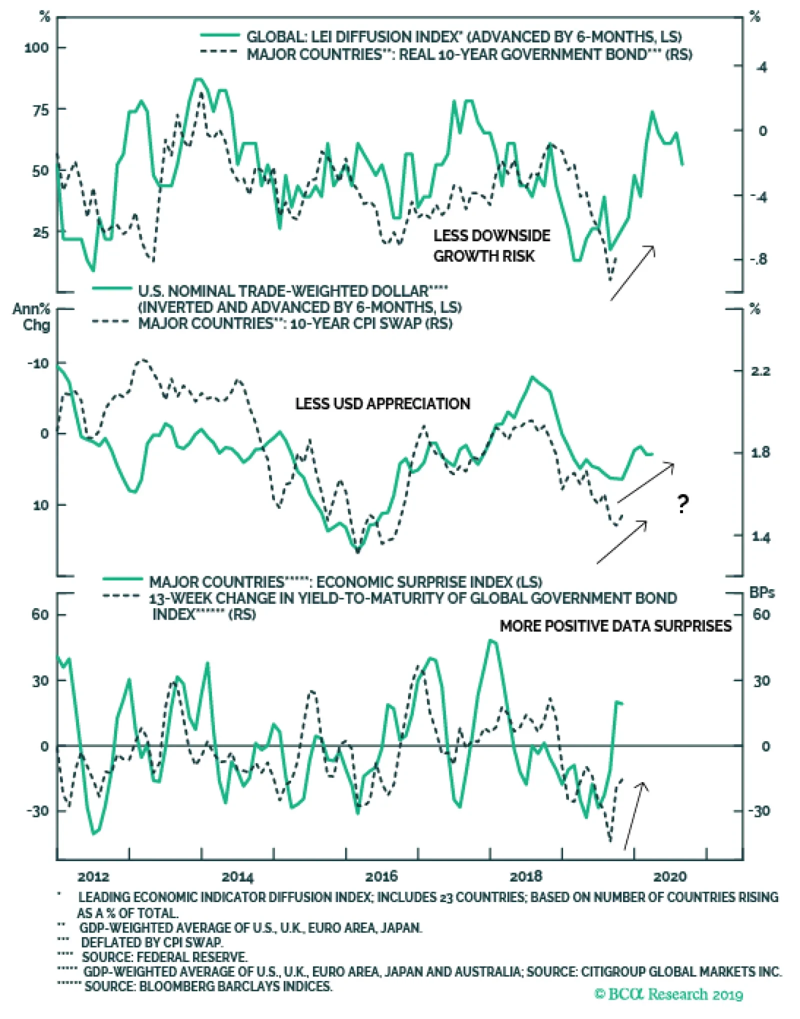
The timing of the bottoming of yields in the major developed markets (DM) should not be surprising, given the more bond-bearish turn of reliable leading directional yield indicators. The diffusion index of our global leading economic indicator (LEI), which leads the real (ex-inflation expectations) component of DM bond yields by twelve months, is at an elevated level (Chart 2). At the same time, the slowing of the annual rate of growth in the trade-weighted U.S. dollar, which leads 10-year DM CPI swap rates by around six months, is signaling that bond yields have room to increase from the inflation expectations side. Finally, the rising trend of positive data surprises for the major DM countries is also pointing to higher yields. Breaking it down at the country level, the pickup in DM 10-year bond yields since the 2019 lows has been widespread (Charts 3 & 4). The range of yield increases is as low as +16bps in Japan, where the Bank of Japan (BoJ) is pursuing a yield target, to +46bps in Canada where the economy and inflation are both accelerating. Chart 3Pricing Out Some Expected Rate Cuts …
Pricing Out Some Expected Rate Cuts ...
Pricing Out Some Expected Rate Cuts ...
Chart 4… Across All Developed Markets
... Across All Developed Markets
... Across All Developed Markets
The increase in yields has also occurred alongside reduced expectations for easier monetary policy. Our 12-month discounters, which measure the expected change in short-term interest rates priced into Overnight Index Swap (OIS) curves, show that markets have partially priced out some (but not all) expected rate cuts in all major DM countries. The Three Things That Have Changed For Global Bond Markets So what has changed to trigger a reduction in rate cut expectations and an increase in global yields? The bond-bullish narrative that we refer to in the title of this report can be broken down into the following three elements, which have all turned recently: Slowing global growth (now potentially bottoming) Chart 5Global Growth Bottoming Out
Global Growth Bottoming Out
Global Growth Bottoming Out
Current global growth is still trending lower, when looking at measures like manufacturing PMIs or sentiment surveys like the global ZEW index. Forward-looking measures like our global LEI, however, have been moving higher in recent months, suggesting that a bottom in the PMIs may soon unfold (Chart 5). We investigated that improvement in our global LEI in a recent report and concluded that the move higher was focused almost exclusively within the emerging market (EM) sub-components that are most sensitive to improving global growth.1 This fits with the improvement shown in the OECD LEI for China, a bottoming of the annual growth rate of world exports, and the general acceleration of global equity markets – the classic leading economic indicator. Rising political uncertainty (now potentially fading) The U.S.-China trade war (including the implications for the upcoming 2020 U.S. presidential election) and the U.K. Brexit saga have been the main sources of bond-bullish political uncertainty over the past several months. Yet recent developments have helped reduce the odds of the most negative tail risk outcomes, providing a bit of a boost to global bond yields. The U.S. and China have agreed (in principle) to a “phase one” trade deal that, at a minimum, lowers the chances of a further escalation of the trade dispute through higher tariffs. Meanwhile, the momentum has shifted towards a potential final Brexit agreement between the U.K. and European Union that can avoid an ugly no-deal outcome. Our colleagues at BCA Research Geopolitical Strategy believe that developments are likely to continue moving away from the worst-case scenarios, given the constraints faced by policymakers.2 U.S. President Donald Trump is now in full campaign mode for the 2020 elections and needs a deal (of any kind) to deflect criticism that his trade battle with China is dragging the U.S. economy into recession. Already, there has been a sharp decline in income growth for workers in swing states that could vote for either party’s candidate in next year’s election (Chart 6). Trump cannot afford to lose voters in those states, many of which are in the U.S. industrial heartland (i.e. Ohio, Michigan) that helped put him in the White House. In other words, he is highly incentivized to turn down the heat on the trade war or else face a potential loss next November. While these political uncertainties have not been fully resolved by these latest developments, the shift in momentum away from worst-case scenarios has likely been enough to reduce the safe-haven bid for DM government bonds, helping push yields higher. Meanwhile, China is facing a slowing economy and rising unemployment, but with reduced means to fight the downtrend given high private sector debt that has impaired the typical response between easier monetary conditions and economic activity (Chart 7). While the Chinese government does not want to be seen as caving in to U.S. pressure on trade policy, its desire to maintain social stability by preventing a further rise in unemployment from the trade war provides a powerful incentive to try and ratchet down tensions with the U.S. Chart 6Political Reasons For Trump To Retreat On Trade
Political Reasons For Trump To Retreat On Trade
Political Reasons For Trump To Retreat On Trade
In the U.K., a no-deal Brexit is an economically painful and politically unpopular outcome that would severely damage the re-election chances of Prime Minister Boris Johnson and his Conservative party. Thus, even a hard-line Brexiteer like Johnson must respond to the political constraints forcing him to try and get a Brexit deal done (Chart 8). Chart 7Economic Reasons For China To Retreat On Trade
Economic Reasons For China To Retreat On Trade
Economic Reasons For China To Retreat On Trade
Chart 8Political Reasons To Retreat On A No-Deal Brexit
Political Reasons To Retreat On A No-Deal Brexit
Political Reasons To Retreat On A No-Deal Brexit
While these political uncertainties have not been fully resolved by these latest developments, the shift in momentum away from worst-case scenarios has likely been enough to reduce the safe-haven bid for DM government bonds, helping push yields higher. Bull-flattening pressure on yield curves (now turning into moderate bear-steepening) The final leg down in bond yields in August had a technical aspect to it, fueled by the demand for duration and convexity from asset-liability managers like European pension funds and insurance companies. Falling yields act to raise the value of liabilities for that group of investors, forcing them to rapidly increase the duration of their assets to match the duration of their liabilities (the technique used to limit the gap between the value of assets and liabilities). That duration increase is carried out by buying government bonds with longer maturities (and higher convexity), but also through the use of interest rate derivatives like long maturity swaps and swaptions. The end result is a bull flattening of yield curves (both for government bonds and swaps) and a rise in swaption volatility (i.e. the price of swaptions). Those dynamics were clearly in play in August after the shocking imposition of fresh U.S. tariffs on Chinese imports early in the month. Bond and swaption volatilities spiked, and bond/swap yield curves bull-flattened, in both Europe and the U.S. (Chart 9). That effect only lasted a few weeks, however, and volatilities have since declined and curves have steepened. This suggests that the “convexity-buying” effect has run its course and is now starting to work in the opposite direction, with asset-liability managers looking to reduce the duration of their assets as higher yields lower the value of their liabilities. This is putting some upward pressure on longer-maturity global bond yields. Chart 9Signs Of Reduced Convexity-Related Bond Buying
Signs Of Reduced Convexity-Related Bond Buying
Signs Of Reduced Convexity-Related Bond Buying
Chart 10Bull-Flattening Yield Curve Pressures Easing Up A Bit
Bull-Flattening Yield Curve Pressures Easing Up A Bit
Bull-Flattening Yield Curve Pressures Easing Up A Bit
Chart 11Fed & ECB Actions Should Help Steepen Up Curves
Fed & ECB Actions Should Help Steepen Up Curves
Fed & ECB Actions Should Help Steepen Up Curves
The steepening seen so far must be put in context, however, as yield curves remain very flat across the DM world (Chart 10). Term premia on longer-term bonds remain very depressed, although those should start to increase as global growth stabilizes and the massive safe-haven demand for global government debt begins to dissipate. Some pickup in inflation expectations would also help impart additional bear-steepening momentum to yield curves – a more likely result now that the Fed and ECB have both cut interest rates and, more importantly, will start provide additional monetary easing by expanding their balance sheets (Chart 11). Bottom Line: The factors that have driven bond yields lower throughout 2019 – slowing growth, rising uncertainty, demand for safe assets and dovish monetary policy expectations – have all started to turn in a more bond-bearish direction. Reviewing Our Recommended Bond Allocations In light of these shifting global trends described above, the fixed income investment implications are fairly straightforward: Yields are rising around the world, suggesting that the current move is a shift higher driven by non-country-specific factors like more stable future global growth prospects. Duration: A moderate below-benchmark overall duration stance is warranted for global fixed income portfolios, with yields likely to continue drifting higher over at least the next six months. A big surge in yields is unlikely, as central banks will need to see decisive evidence that global growth is not only bottoming, but accelerating, before shifting away from the current dovish bias. Given the reporting lags in the economic data, such evidence is unlikely to appear until the first quarter of 2020 at the earliest. Yet given how flat yield curves are across the DM government bond markets, the trajectory of forward rates is quite stable relative to spot yield levels, making it much easier to beat the forwards by positioning for even a modest yield increase. Country Allocation: Yields are rising around the world, suggesting that the current move is a shift higher driven by non-country-specific factors like more stable future global growth prospects. In that case, using yield betas to the “global” bond yield is a good way to consider country allocation decisions within a fixed income portfolio. We looked at those yield betas in an August report, using Bloomberg Barclays government bond index data for the 7-10 year maturity buckets of individual countries and the Global Treasury aggregate (Chart 12).3 The rolling 3-year betas were highest in the U.S. and Canada, making them good countries to underweight within a global government bond portfolio in a rising yield environment. The yield betas were lowest in Japan, Germany and Australia, making them good overweight candidates. The U.K. was a unique case of having a relatively high historical yield beta prior to the 2016 Brexit referendum and a lower yield beta since then - making the U.K. allocation highly conditional on the resolution of the Brexit uncertainty. Spread Product Allocation: The backdrop described in this report, where global growth is bottoming out but where central banks maintain a dovish bias, is a perfect sweet spot for global spread product like corporate bonds and Peripheral European government debt. Thus, an overweight stance on overall global spread product versus governments is warranted. The backdrop described in this report, where global growth is bottoming out but where central banks maintain a dovish bias, is a perfect sweet spot for global spread product like corporate bonds and Peripheral European government debt. With regards to our current strategic fixed income recommendations and model bond portfolio allocations, we already have much of the positioning described above in place. We are below-benchmark on overall duration, underweight higher-beta U.S. Treasuries; overweight government bonds in lower-beta Germany, France, Japan and Australia (Chart 13); overweight investment grade corporate bonds in the U.S., euro area and U.K.; and overweight high-yield corporate bonds in the U.S. and euro area. Chart 12Favor Lower-Beta Government Bond Markets
Favor Lower-Beta Government Bond Markets
Favor Lower-Beta Government Bond Markets
There are areas where our positioning could change, however. Chart 13Lower-Beta Laggards Should Start To Outperform
Lower-Beta Laggards Should Start To Outperform
Lower-Beta Laggards Should Start To Outperform
In terms of government bonds, we are currently overweight the U.K. and neutral Canada. A final Brexit deal would justify a downgrade of Gilts to at least neutral, if not underweight, as the Bank of England has signaled that rate hikes would be justified if the Brexit uncertainty was resolved. A downgrade of higher-beta Canadian government debt to underweight could also be justified, although the Bank of Canada is not signaling that a change in monetary policy (in either direction) is warranted. For now, we will hold off on any change to our U.K. stance, as it is now likely that there will be another extension of the Brexit deadline beyond October 31. As for Canada, we remain neutral for now but will revisit that stance in an upcoming Weekly Report. With regards to spread product, we are only neutral EM USD-denominated sovereign and corporate debt, as well as Spanish sovereign bonds; and underweight Italian government debt. An EM upgrade to overweight would require two things that are not yet in place: a weaker U.S. dollar and accelerating Chinese economic growth. Chart 14Stay Overweight Corporates In The U.S. & Europe
Stay Overweight Corporates In The U.S. & Europe
Stay Overweight Corporates In The U.S. & Europe
As for Peripheral governments, we have preferred to be overweight European corporate debt relative to sovereign bonds in Italy and Spain. The recent powerful rally in the Periphery, however, has driven the spreads over German bunds in those countries down to levels in line with corporate credit spreads (Chart 14). We will maintain these allocations for now, but will investigate the relative value proposition between euro area Peripheral sovereigns and corporates in an upcoming report. Bottom Line: Maintain a moderate below-benchmark stance on aggregate bond portfolio duration. Favor lower-beta countries with central banks that are more likely to stay relatively dovish as global yields drift higher, like core Europe, Australia and Japan. Stay overweight corporate bonds versus government debt in the U.S. and Europe, both for investment grade and high-yield. Maintain just a neutral stance on EM USD-denominated spread product, but look to upgrade if global growth improves further and the USD begins to weaken. Robert Robis, CFA Chief Fixed Income Strategist rrobis@bcaresearch.com Footnotes 1 Please see BCA Research Global Fixed Income Strategy Weekly Report, “What Is Driving The Improvement In The BCA Global Leading Economic Indicator?”, dated October 2, 2019, available at gfis.bcaresearch.com. 2 Please see BCA Research Geopolitical Strategy Weekly Report, “Five Constraints For The Fourth Quarter”, dated October 11, 2019, available at gps.bcaresearch.com. 3 Please see BCA Research U.S. Bond Strategy/Global Fixed Income Strategy Weekly Report, “Where’s The Positive Carry In Bond Markets?", dated August 20, 2019, available at usbs.bcaresearch.com and gfis.bcaresearch.com. Recommendations The GFIS Recommended Portfolio Vs. The Custom Benchmark Index
Cracks Are Forming In The Bond-Bullish Narrative
Cracks Are Forming In The Bond-Bullish Narrative
Duration Regional Allocation Spread Product Tactical Trades Yields & Returns Global Bond Yields Historical Returns
Highlights Given that rising crop yields have been the main vehicle through which global supply of agricultural commodities grew to meet expanding demand, the risks posed to yields due to climate change are non-trivial. The impact of climate change will manifest itself in the form of two simultaneous trends: the gradual rise in temperatures alongside more frequent and severe weather events. While the latter will threaten immediate supply, the former is a slower moving process, and its net negative impact is unlikely to manifest before 2030. The implications of climate change on agriculture producers are non-uniform. Low-latitude countries with economies that are highly dependent on the agriculture sector will suffer most. Expect greater volatility in agriculture prices as the frequency of weather events will raise uncertainty. Feature The steady expansion of global population and rising per-capita calorie consumption has directly translated to growing demand for agricultural products of all types. However, these demand-side pressures increasingly will be met with disruptions to global supply of agricultural commodities, as the impact of climate change raises uncertainty. In any given year, the aggregate decisions of farmers all over the world – i.e., the choice of which crops to plant and how much acreage to dedicate to each crop – determine the supply and market prices of ags. In this competitive market, each farmer attempts to maximize his or her welfare by planting the crops that are expected to yield the greatest profit. Chart 12010/11 Shock Highlights Ag Vulnerability To Weather
2010/11 Shock Highlights Ag Vulnerability To Weather
2010/11 Shock Highlights Ag Vulnerability To Weather
The collective action of these producers in reaction to perceived demand generally leads to stable prices, especially for staple commodities such as grains and oilseeds, which differ from industrial commodities in that they are not highly correlated with global business cycles. Demand trends are long-term and slow moving, and typically do not result in abrupt price pressures, as farmers have time to adjust and adapt to changing consumer preferences. Unforeseen, weather-induced supply-side shocks, therefore, are the main source of sudden price changes in ag markets. Such a shock was dramatically on display during the drought-induced crop failures in major grain and cereal producing regions in the most recent global food crisis of 2010/11. While this massive supply shock was not the first of its kind (Chart 1, on page 1), it highlighted the vulnerability of ag markets to weather risks and specifically the evolving environment under climate change. A 2019 study quantifies the impact of shifting weather patterns on the agricultural market, finding that year-to-year changes in climate factors during the growing season explain 20%-49% of change in corn, rice, soybean, and wheat yields, with climate extremes accounting for 18%-43% of this variation.1 In theory, the impact can manifest in several ways, sometimes contradictory: Extreme weather events: An increase in the frequency and intensity of droughts or floods which threaten to wipe out crops or reduce yields, creating unpredictable supply shocks. The gradual rise in temperature: Each crop has cardinal temperatures – defined by the minimum, maximum and optimum – that determine its boundaries for growth. Increases in temperatures induced by global warming may push the boundary, reducing yields in some regions. Changes in precipitation patterns: In many areas precipitation is projected to increase – both in short bursts and over longer periods. This will lead to greater soil erosion resulting in deterioration in the quality of soil. In other regions, precipitation will decrease, and drought is expected to become more frequent.2 Moreover, the interaction of these factors – along with other region-specific variables – will amplify the impact on crops: Rising temperatures and greater precipitation will result in greater amounts of water in the atmosphere, producing increased water vapor and greater cloud cover. This will reduce solar radiation, and will harm crop productivity. Elevated atmospheric carbon dioxide and CO2 fertilization: Greater CO2 concentrations brought on by continued growth in air pollution are positive for crops as they stimulate photosynthesis and plant growth. However, the impact differs across crops with plants such as soybeans, rice and wheat set to benefit relatively more than plants such as corn.3 Moreover, elevated atmospheric CO2 levels can help crops respond to environmental stresses and reduce yield losses due to ozone and crop water loss through partial stomatal closure and a reduction in ozone penetration into leaves. Temperature changes and the magnitude and intensity of precipitation impact soil moisture and surface runoff. Indirect effects of climate change – weeds, pests and pathogens – also present challenges as they require changes to management practices and may raise farming costs required. The impact of climate change on agriculture markets is already evident in increasing intensity and frequency of extreme weather events. The confluence of these factors, and the region- and crop-specific nature of these variables, makes it impossible to estimate the impact of evolving climate conditions on ag products with great accuracy. Nevertheless, our research suggests that the impact of climate change on ag markets will create opportunities in this evolving and highly uncertain market. Abrupt Shocks Amid Gradual Warming: The Long And Short View The impact of climate change on agriculture markets is already evident in the increasing intensity and frequency of extreme-weather events such as heatwaves, floods, and droughts. Charts 2A, 2B, and 2C, illustrate the impact of major weather events in crop-producing regions of the U.S. on yields, production and acreage for the crop year in which the events took place. Chart 2AExtreme Weather Events Reduce U.S. Corn Supplies …
Extreme Weather Events Reduce U.S. Corn Supplies
Extreme Weather Events Reduce U.S. Corn Supplies
Chart 2B… Soybean Supplies …
Extreme Weather Events Reduce U.S. Soybean Supplies
Extreme Weather Events Reduce U.S. Soybean Supplies
Chart 2C… And Wheat Supplies In A Big Way
Extreme Weather Events Reduce U.S. Wheat Supplies In A Big Way
Extreme Weather Events Reduce U.S. Wheat Supplies In A Big Way
Chart 3Climate-Induced U.S. Supply Shocks Associated With Price Spikes
Climate-Induced U.S. Supply Shocks Associated With Price Spikes
Climate-Induced U.S. Supply Shocks Associated With Price Spikes
While the individual losses are a function of the magnitude of the event, the events highlighted translate to a 16%, 10%, and 7% decline in corn, soybean, and wheat yields, respectively. These supply disruptions generally do not extend beyond the event year, as the new crop year offers farmers a clean slate to raise output and maximize profits. Given that the U.S. is a major global supplier of these crops, extreme weather events and the subsequent supply reductions lead to non-negligible price pressures (Chart 3). While crop conditions thus far have failed to deteriorate in trend (Chart 4), greater frequency and intensity of weather events raise the probability of a decline in overall crop and could lower supply. Chart 4Crop Conditions Have Generally Held Up
Climate Change Special Series: An Introduction
Climate Change Special Series: An Introduction
Expanding the analysis to other major crop-producing regions of the world, we find that once again, extreme-weather events are associated with a decline in yields and production in the corresponding crop year (Chart 5). This exercise also indicates that the impact of droughts is significantly more pronounced than the impact of floods.4 While the weather-induced supply shocks described above are unpredictable, abrupt, and have an immediate impact on output and prices, the gradual warming of temperatures is a slow-moving process. Consequently, the impact will manifest in the form of gradual changes that are difficult to capture and quantify, especially given the mitigating effect of CO2 fertilization – i.e., higher yields resulting from higher CO2 in the atmosphere. Nonetheless, rising temperatures will become a serious risk in crop-planting regions both in the U.S. and globally (Chart 6). While rising temperatures are expected to bring about increasingly more wide-ranging supply disruptions (Chart 7), the net impact over the coming decade is not a clear negative. Chart 5Weather Events, Especially Droughts, Hurt Global Supplies
Climate Change Special Series: An Introduction
Climate Change Special Series: An Introduction
Chart 6Rising Global Temperatures Will Pose A Serious Risk …
Climate Change Special Series: An Introduction
Climate Change Special Series: An Introduction
Chart 7… Especially Above The 2°C Mark
Climate Change Special Series: An Introduction
Climate Change Special Series: An Introduction
One study expects the positive impact of CO2 fertilization on yields to overwhelm the negative effect of rising temperatures over the coming decade (Table 1). Elsewhere, studies forecast different responses, with some predicting incremental yield gains over the coming decade before temperatures rise to levels that overwhelm the benefits of greater CO2. Similarly, according to the FAO’s assessment, the net negative impact of climate change on global crop yields will only become apparent with a high degree of certainty post-2030.5 Table 1Estimates For The Response Of Global Average Crop Yields To Warming And CO2 Changes Over The Next Decades
Climate Change Special Series: An Introduction
Climate Change Special Series: An Introduction
Bottom Line: Given that rising crop yields have been the main vehicle through which global ag supply grew to meet expanding demand, the risks posed to yields due to climate change are non-trivial. Supply disruptions generally do not extend beyond the event year, as the new crop year offers farmers a clean slate to raise output and maximize profits. The impact will manifest itself in the form of two simultaneous trends: the gradual rise in temperatures alongside more frequent and severe weather events. While the latter will threaten immediate supply, the former is a slower moving process, and its net negative impact is unlikely to manifest before 2030. The Winners … And Losers Rising temperatures are expected to result in a negligible impact on ag markets over the coming decade; yet this finding is not uniform across all regions. The FAO study cited above finds that by 2030, the projected impact on crop yields will be slightly net negative in developing countries. However, in developed countries, the effect will be net positive. In terms of global supply, the impact of climate change over the coming decade is expected to remain relatively contained, affecting certain regions at various times without causing major global disruptions. That said, as global warming and extreme weather persist, the ramifications will begin to extend beyond individual regions, and will cause supply shocks on a global scale. In part, this can be explained by a greater potential for net reductions in crop yields in warmer, low-latitude areas and semi-arid regions of the world.6 This non-uniform impact will create relative winners and losers. Producers located in temperate regions – where climate change does not yet pose as serious a threat – are set to profit from their increased role in global supply. Conversely, tropical regions are much more vulnerable to climate change. This is especially true for those whose economies are highly dependent on agriculture (Chart 8). Chart 8Agricultural Economies In Tropical Regions Are Most Vulnerable
Climate Change Special Series: An Introduction
Climate Change Special Series: An Introduction
On net, the overall economies of DM countries – which generally are not economically dependent on agriculture and are located in northern regions – will be relatively more insulated from the impact of climate change on the agriculture sector. Aside from the impact on producers, the implications on consumers are also region-dependent. Clearly the direct impact of climate change on global agriculture will be higher food prices, which directly impacts the food component of inflation generally. As a result, consumers who spend a large share of their income to food – generally consumers in lower income countries – will be hardest hit (Chart 9). Chart 9Higher Food Prices Disproportionately Hurt Consumers In Lower Income Countries
Climate Change Special Series: An Introduction
Climate Change Special Series: An Introduction
In theory, a food supply shock is transitory, and given that food is usually excluded from core inflation gauges targeted by central banks, monetary policy should not react to these price spikes. All the same, aside from this direct impact on inflation, food inflation can also pass-through into other components of the CPI basket, for example through wage pressures or inflation expectations. This would lead to a more persistent impact on core inflation, forcing policy makers to react to these transitory forces, complicating the monetary policy response function for these countries. Given that inflation expectations are less well-anchored in lower income economies and that food makes up a larger share of consumption expenditures in these economies, they are most vulnerable to weather-induced food shocks. Chart 10Subsidies Partially Insulate Against International Shocks
Climate Change Special Series: An Introduction
Climate Change Special Series: An Introduction
In countries where food prices are highly subsidized, the impact of higher global food prices will not immediately translate to higher domestic prices. This explains why there is no one-to-one relationship between global food prices and domestic food prices (Chart 10). Instead, the higher prices are absorbed by the governments, resulting in an expansion in government expenditures. This distorts the local food market, as it prevents demand from adjusting to the higher prices, and could potentially result in an undershoot in inventories that makes global markets even more vulnerable to further supply shocks. Bottom Line: The implications of climate change on ag producers are non-uniform. While higher-latitude regions are set to benefit, at least in the short-run, low-latitude countries with economies that are highly dependent on the agriculture sector will suffer most. On the consumer side, individuals who spend a large share of their income on food are set to suffer most. While consumers in countries that subsidize the crops will be protected from the immediate inflation risk, they may feel a delayed impact due to an increase in budget expenditures needed to cover the larger import bill. Mitigation Efforts While the potential impact of climate change on the agriculture sector can be large, it will be at least partially managed through adoption of mitigation policies (Diagram 1). Diagram 1Adaptation Reduces Vulnerability
Climate Change Special Series: An Introduction
Climate Change Special Series: An Introduction
A key question in determining the extent of this behavior is whether warming temperatures and the increased occurrence and intensity of extreme events will be sufficient to justify a major acceleration of investment in agriculture. These efforts would range from simple management changes on the part of farmers to technological advances that raise the productivity of farming or reduce the vulnerability of farmers to climate change. For example, farmers across the U.S. have been planting corn and soybeans earlier in the spring, resulting in an advancement in planting dates (Chart 11). The earlier planting has also been accompanied by a longer growing season with the average number of days in the season increasing. Farmers are also adapting by altering their decisions on which crops to plant. For example, since soybean and corn are planted in many of the same regions of the U.S., farmers often plant more soybeans than corn when experiencing weather shocks. Chart 11Weather Events, Especially Droughts, Hurt Global Supplies
Climate Change Special Series: An Introduction
Climate Change Special Series: An Introduction
The agriculture sector is also using more efficient machinery that can plant and harvest crops much faster as well as developing heartier seeds and more potent fertilizers. In turn, farmers will alter their decision making by selecting crop varieties or species that are more resistant to heat and drought. Or they will change fertilizer rates, amounts and timing of irrigation, along with other water-management techniques. Farmers also are making wider use of integrated pest and pathogen management techniques, in order to raise the effectiveness of pest, disease, and weed control. Given that the number of firms in the agriculture sector are fewer in developed markets than in the rest of the world, management decisions can be more easily implemented in the former. Farmers across the U.S. have been planting corn and soybeans earlier in the spring, resulting in an advancement in planting dates. On the other hand, emerging market countries where ag output is driven by numerous individual farmers will have a more difficult time implementing policies. Individual farms may not have the means to support themselves, which raises the potential impact of climate change. What is more, climate-change mitigation efforts may require projects, programs, or funds set aside by the government to support these efforts. This is more likely to occur in wealthier developed countries. Bottom Line: Adaptation and mitigation measures on the part of farmers have the potential to reduce the impact of climate change. That said, farmers in richer countries with the funds and institutions in place to support the ag sector likely will fare better. Investment Implications Over the coming decade, the ramifications of climate change are likely to be contained to a regional level. Although global supply will be vulnerable to regional disruptions, the impact will, in part, be mitigated by inventories, which have been rising for years. These stocks will create a buffer against unpredictable supply shocks (Chart 12). Chart 12Higher Inventories Needed To Buffer Against Unpredictable Shocks
Climate Change Special Series: An Introduction
Climate Change Special Series: An Introduction
However, given that the global soybean market resembles an oligopoly with Brazil, the U.S., and Argentina accounting for 81% of global supply, global soybean prices will be more vulnerable to supply events in these regions than other crops (Chart 13). Chart 13Soybeans Most Vulnerable To Shocks Affecting Major Producers
Climate Change Special Series: An Introduction
Climate Change Special Series: An Introduction
At the other end of the spectrum, global wheat markets will be relatively more insulated from isolated weather events impacting any one major producer as each of these regions contributes a relatively small share to global wheat output. This analysis also finds that yields and supply generally recover in the crop year following an extreme climate event. This implies that while the extent of damage from these events can be severe, they are not persistent unless the increasing frequency of extreme events leads to a secular change. Aside from the price impact, the weather and temperature changes will manifest in the form of greater volatility in supply, translating to greater price volatility. Options-implied volatilities for corn, wheat and soybeans have been on a general downtrend since the two major global food scares in 2007/08 and 2010/11 (Chart 14). We expect the trend to reverse going forward as the frequency of weather events will create greater price uncertainty. We summarize the findings of this report in Table 3 (Appendix, on page 16). Chart 14Volatility Will Go Up
Climate Change Special Series: An Introduction
Climate Change Special Series: An Introduction
Roukaya Ibrahim Editor/Strategist RoukayaI@bcaresearch.com Jeremie Peloso Research Analyst JeremieP@bcaresearch.com Amr Hanafy Research Associate AmrH@bcaresearch.com Hugo Bélanger Senior Analyst HugoB@bcaresearch.com Isabelle Dimyadi Research Associate Isabelled@bcaresearch.com Appendix Table 2Extreme Weather Events In The U.S.
Climate Change Special Series: An Introduction
Climate Change Special Series: An Introduction
Table 3Summary Table
Climate Change Special Series: An Introduction
Climate Change Special Series: An Introduction
Footnotes 1 Please see Vogel et al, The effects of climate extremes on global agricultural yields, Environ. Res. Lett 14 054010, 2019. 2 As a consequence of greenhouse gas emissions precipitation is expected to increase in high altitude regions such as much of the U.S. and decrease in subtropical regions such as the southwest U.S., Central America, southern Africa, and the Mediterranean basin. 3 Plants can be broken down into either C3 or C4 based on the way they assimilate atmospheric CO2 into different physiological components. While rising CO2 causes C3 plants to raise the rate of photosynthesis and reduce the respiration rate, C4 plants do not experience a rise in photosynthesis since photosynthesis is already saturated. For example, studies show that soybean yields increased 12%-15% under 550 ppm vs. 370 ppm CO2 concentrations while corn experienced negligible yield increases. 4 Please see Lesk C., P. Rowhani, and N. Ramankutty, Influence of extreme weather disasters on global crop production, Nature, 529(7584), 84-87, 2016. 5 Please see The State Of Food And Agriculture: Climate Change, Agriculture, And Food Security, Food and Agriculture Organization of the United Nations, 2016. 6 Please see Stevanovic et al., The impact of high-end climate change on agricultural welfare, Sci-Adv 2(8), 2016.
Highlights As an introduction to a series of BCA Special Reports on the investment consequences of climate change, we review the science around the subject and suggest a framework for analyzing its implications. The scientific consensus is that global warming is a reality and most likely human-induced. However, the uncertainty around the magnitude of the impact of climate change is large. The consequences of climate change are delayed, uncertain and global. But, for investors, the prudent course of action is to accept the scientific consensus – and the impact it will have on policymakers – and hedge or invest appropriately. Feature Chart 1Climate Change Global Perception
Climate Change Special Series: An Introduction
Climate Change Special Series: An Introduction
Bank of England Governor Mark Carney has called climate change “the tragedy of the horizon.” It is now perceived as a major threat across the globe (Chart 1). As such, it is essential to assess its macro and market consequences. In this introduction to our Climate Change Special Series, we review the existing literature and suggest a framework to assess the market relevance of this phenomenon. Going forward, we will produce a series of market-driven reports designed to help investors both mitigate the risk to their portfolios and identify opportunities arising from climate change. We intend to cover topics such as green financing, energy, and the geopolitical aspect of climate change, just to cite a few. These reports will incorporate both quantitative and qualitative analysis to generate actionable investment recommendations. What Is Climate Change? Climate science is not new. The initial understanding of the effect of heat-trapping gases on global temperature dates back to Joseph Fourier’s early 1800s study of planetary temperature. Subsequent research showed the importance of the greenhouse effect, a phenomenon whereby greenhouse gas molecules (e.g. CO2, CH4, N2O) absorb infrared radiation emitted from Earth before reemitting it in all directions, including back to the Earth’s surface, thus making it harder for this energy to leave the planet. This excess of energy stored in the planet, above its normal energy balance, causes temperature increases. The distribution of environmental damages caused by global warming will not be uniform around the world. The rate of warming and other climate changes will differ across regions due to climate processes and feedbacks linked to local conditions.1 Regardless, up to 14% of the global population will experience above 2°C (3.6°F) warming – a level seen by scientists as a trigger for permanent damages and changes – even if the increase in global mean surface temperature (GMST) were limited to 2°C (3.6°F) by 2100 (CarbonBrief, 2018). The consequences of climate change are delayed, uncertain and global. Even under the maximum policy effort scenario, studies assign 60% odds to an increase greater than 2°C (3.6°F) (Nordhaus, 2018). The longer policymakers, companies and investors delay tackling this issue, the less likely the world will stay below the 2°C threshold and the more rapid and abrupt the transition to a low-carbon economy will eventually be. A sudden transition will be more disruptive to the economy and damaging to investors. Defining The Issue: The Earth’s Atmosphere As A Global Common The Earth’s atmosphere - specifically its function as a sink for CO2 and other greenhouse gases (GHG) - falls within the problem of the global commons.2 It is a natural resource requiring global cooperation for its sustainable use and provision. Problematically, the consequences of climate change are delayed, uncertain and global. Delayed because the burden of climate change policies mainly falls on current generations, whereas the benefits of lower climate damage accrue to future generations, leading every generation to think it can survive the issue and let the next generations handle it. Uncertain because the list of harms from climate change lengthens with the advance in climate-science studies. We learn more and more about the extent to which human activities are at fault and the extent of the damage that will befall the planet. Global because it does not matter whether the emissions take place in China, Europe, or the U.S. since GHG mix immediately once in the atmosphere. In that sense, it is a collective-action problem in which every country’s interest is to shift the abatement costs onto its neighbor. The global aspect is crucial. The optimal emission level of one country does not follow the global social optimal. Hence, every country has an incentive to emit as much GHG as possible now, before any consequences occur (Combes, 2016). What We Know So Far: Historical Data Both climate-alarmist and climate-denier groups have captured the public debate.This polarization clouds the underlying facts about current trends and the difference between what is unlikely, likely, or very likely to happen. The resulting lack of consensus will lead to over- or under-adaptation by the various economic agents, depending on their interests. FACT 1: GLOBAL WARMING IS A REALITY Anthropogenic Greenhouse Gas Emissions - Emissions of carbon dioxide (CO2), methane (CH4), and nitrous oxide (N2O) have risen steadily since the industrial revolution and at a brisk pace relative to the previous 12,000 years (Chart 2). Chart 2GHG Global Emissions
GHG Global Emissions
GHG Global Emissions
Global Mean Surface Temperature - It rose by an estimated 1°C (1.8°F) from 1901 to 2016. According to NASA data, the 10 warmest years recorded in the past 139 years all occurred after 2005 (Chart 3). Chart 3Global Land And Ocean Temperature
Global Land And Ocean Temperature
Global Land And Ocean Temperature
Global Mean Sea level - It has risen by an estimated 20.3cm (8 inches) since 1900 due to the expansion of waters and meltwater from shrinking ice sheets. Almost half of this rise happened in the last 25 years (Chart 4). Glacier and Ice Sheet - The melting of ice sheets will reduce the earth’s reflectivity, accelerating the warming process (Chart 5). The record low of sea ice extent in the Arctic and Antarctic was observed in 2012 and 2017, respectively. Chart 4Global Mean Sea Level
Global Mean Sea Level
Global Mean Sea Level
Chart 5Glacier And Ice Sheet
Glacier And Ice Sheet
Glacier And Ice Sheet
Precipitation - Historical changes in precipitation are much more volatile and region-specific than temperature and sea level changes. Moreover, there is a lack of data covering the period before 1951, which leads to low confidence in estimates of precipitation for this period and medium confidence post-1951. Annual average precipitation for global land areas increased slightly over the period 1901–2008, and the magnitude of observed changes varies across different datasets (Hartmann, 2013). Extreme Weather Events - These are defined, in a meteorological sense, as events at the “edges of the complete range of weather experienced in the past.” The frequency and severity of extreme weather events has been linked to global warming (Table 1) (Scott, 2016). Table 1Extreme Weather Events (1950 - Present)
Climate Change Special Series: An Introduction
Climate Change Special Series: An Introduction
FACT 2: CLIMATE CHANGE IS HUMAN-INDUCED The Intergovernmental Panel on Climate Change (IPCC) – considered the world’s most authoritative scientific body on climate change – concluded in 2013 that the probability that global warming was human-induced was at least 95% (Table 2). Table 2Evolution Of The Assessments Of Human Influence On Climate Change
Climate Change Special Series: An Introduction
Climate Change Special Series: An Introduction
Chart 6Global Warming & Global GHG Emissions
Global Warming & Global GHG Emissions
Global Warming & Global GHG Emissions
Since the late nineteenth century, GHG emissions – mainly CO2 – and global land and ocean mean temperature have shared a common steep upward trend (Chart 6). A recent study by Mann et al. estimates that in the absence of GHG emissions, the odds that 13 out of the 15 warmest years ever measured would all have happened in the current century are extremely small.3 More recently, a report by the National Academies of Sciences, Engineering, and Medicine (NASEM) concluded that “[I]n many cases, it is now possible to make and defend quantitative statements about the extent to which human-induced climate change has influenced either the magnitude or the probability of occurrence of specific types of events or event classes.” According to most recent peer-reviewed studies, at least 97% of actively publishing climate scientists now accept human-caused climate warming (Cook, 2016). While science is not a matter of popular vote, this level of consensus among experts suggests that for investors the most prudent course of action is to accept the scientific consensus and hedge or invest appropriately. Projections & Assumptions Chart 7Global Emissions Projections
Climate Change Special Series: An Introduction
Climate Change Special Series: An Introduction
Climate economics deals with conditional projections based on unknown probability distributions, implying a high level of uncertainty. The level of confidence around the nearer segments of the projections is relatively elevated. Conversely, at the far end of the projected period, by 2100 for most studies, the uncertainty increases drastically. According to the United Nations Environment Programs’ 2018 Emissions Gap report, the 2°C (3.6°F) target drafted in the Paris Agreement in 2015 would require global emissions to be capped at 40 gigatons of CO2 equivalent by 2030. Throughout our Climate Change Special Series, we will rely on the following assumptions based on the IPCC Fifth Assessment Report (AR5) and the summary estimates from around 150 academic papers, the majority of which were published in 2018 (CarbonBrief, 2018). Anthropogenic Greenhouse Gas Emissions - Global emissions rose in 2017 and are now ~14 GtCO2e above the required level by 2030. Current pledges are insufficient to meet the Paris Agreement’s long-term temperature goals (Chart 7). Key factors driving changes in anthropogenic GHG emissions are mainly economic and population growth. Projections of greenhouse gas emissions vary over a wide range, depending on both socio-economic development and climate policy – which are fundamentally uncertain. Climate economics deals with conditional projections based on unknown probability distributions, implying a high level of uncertainty. The majority of models indicate that scenarios meeting levels similar to RCP2.6 (a scenario that aims to keep global warming likely below 2°C (3.6°F) above pre-industrial temperatures) are characterized by substantial net negative emissions by 2100, on average 2 GtCO2e per year. Chart 8Global Mean Surface Temperature Projections
Global Mean Surface Temperature Projections
Global Mean Surface Temperature Projections
Global Mean Surface Temperature - Under all assessed emission scenarios, surface temperature is projected to rise over the twenty-first century. The change over the 2016-2035 period will be very similar to 1986-2005, and will likely be in the range of 0.3°C to 0.7°C (0.5°F to 1.3°F). Beyond that, the mean temperature rise across IPCC scenarios for 2046-65 and 2081-2100 is estimated to be 1.4°C (2.5°F) and 2.2°C (4°F), respectively (Chart 8). These estimates imply that there will be more frequent hot and fewer cold temperature extremes over most land areas on daily and seasonal timescales. Global Mean Sea Level - It has been established that the likelihood sea levels will rise in more than 95% of the ocean area is very high. Under all IPCC scenarios, the rate of sea level rise will very likely exceed the observed rate during 1971-2010. About 70% of the coastlines worldwide are in fact projected to experience sea level change within +/- 20% of the global mean. Precipitation - There are likely more land regions where the number of heavy precipitation events has increased than where it has decreased. Recent detection of increasing trends in extreme precipitation and discharge in some catchments implies greater risks of flooding at regional scale (medium confidence). These changes will not be uniform, with high latitudes and the equatorial Pacific more likely to experience an increase in annual mean precipitation while many mid-latitude and subtropical dry regions are likely to experience a decrease in mean precipitation. It remains a challenge to determine long-term trends in precipitation for the global oceans. Extreme Weather Events - Projections on extreme weather events can only infer the probability distribution of such events, i.e. more or less likely to happen. With a 1°C (1.8°F) additional warming, risks from extreme weather events are high (medium confidence from IPCC). More importantly, we can say with high confidence that these risks increase progressively with further warming. Embracing Uncertainty The uncertainty around the magnitude of the impact of climate change is large. Yet, bounded uncertainty is informational. We can extract the following important, actionable conclusions: Projections for economic variables are relatively more uncertain than for geophysical variables. The link between GHG emissions and rising temperature is more certain than the level of emissions, output, and damages (Nordhaus, 2018). Therefore, the largest uncertainty comes from economic growth and the level of emissions. We do not rely on estimates of global GDP impacts. On the other hand, it is easier to build scenarios for geophysical variables and obtain investment-relevant information from these projections. Simulating the path of future emission allows us to map this onto future temperature, sea level, and extreme weather variations. Economic models suggest that the higher the uncertainty, the larger the weights on low-probability/high-impact scenarios. This implies a positive risk premium due to risk aversion and favors stricter mitigation policies as insurance to shattering outcomes. As climate models are fine-tuned and continuously point to large damage uncertainty, the desired strength of policy could increase. Win-Win or “no-regrets” investments are the most likely at first.4 The Kaya Identity provides a simple framework to project future GHG emissions to visualize the uncertainty associated with different assumptions. The identity links future emissions to observable macroeconomic variables (see the Appendix for more details): F = P * (G/P) * (E/G) *(F/E) Where F denotes global CO2 emissions from human sources, P represents global population, G equals global GDP, and E is global energy consumption. The identity provides a useful framework for policymakers. To reduce emissions, there needs to be a reduction in one or more of the identity's components. Altering demographic trends and reducing global GDP per capita are very unlikely to happen given the damaging impact it could have – both for individuals and politicians’ careers! At a global level, this leaves us with energy efficiency and carbon intensity of energy as the only key and viable options to reduce CO2 emissions. Why Does It Matter To Investors? Markets are probably still underpricing climate-related risks because the effects only materialize gradually and in the long term – exceeding most investors’ investment horizon. Investors such as pension funds, insurers, wealth managers, and endowments need to be responsive to the threat posed by climate change. They typically have multi-decade time horizons, with portfolio exposure across the global economy. Their increasing interest in Environmental, Social, and Governance (ESG) measures fits well within this context.5 It reflects a need for more transparency and more stringent investing standards. Determining which firms or sectors will either win or lose the “green race” will be of the outmost importance to investors. Businesses are still navigating the financial and operational implications of climate change. To some extent, this can already be assessed based on the readiness of firms and sectors to adapt to a green economy – looking at the number of environmental technology patent applications, for example. Markets are probably still underpricing climate-related risks. The financing needed to mitigate climate change represents yet another opportunity for investors. Green bonds and sustainability-linked debt instruments are more widespread than ever. Sustainable debt issuance reached record levels last year, with a total of $260 billion issued, according to Bloomberg New Energy Finance data. Year-to-date issuance has nearly reached $180 billion. Green bonds offer two main benefits to issuers: corporate branding that sends a strong signal to the market of their commitment to climate change, and a wider investor base. Our series of market-driven reports are intended to both identify the risks and opportunities arising from climate change in order to help investors mitigating the risk to their portfolios. They will rely on the simple framework we present below. Climate Change Framework In future reports in our Climate Change Special Series, we will summarize our findings using a comprehensive analytical framework developed by Batten (2018) to assess the impact of climate change via physical and transition risks with respect to the type of shock induced by each type of risk. Physical Risks Physical risks are the most visible and immediate source of risk to investors and the financial sector. They can be defined as those risks that arise from the interaction between climate-related events and human and natural systems, including their ability to adapt— e.g. the volatility in food prices following a drought or a flood.6 An increase in climate-induced physical risks – such as heat waves, floods and storm – will have a direct effect on insurers. If these risks are uninsured, the deterioration of the balance sheets of affected households and corporations is likely to hurt the banking system. Electrical utilities, real estate and transportation infrastructure are other physical assets at risk of capital losses. Transition Risks Chart 9Public Opinion Of Policy Options To Tackle Climate Change
Climate Change Special Series: An Introduction
Climate Change Special Series: An Introduction
Transition risks can be defined as the risks of economic dislocation and financial losses associated with the transition to a lower-carbon economy. Detrimental effects manifest themselves through three possible channels: Reduced production and consumption of high carbon products, especially energy produced using fossil fuels, potentially leading to stranded assets. Improvement in the energy efficiency of existing products and processes – energy intensity. Moving to low-carbon energy production – that is reducing carbon intensity. Lower energy intensity and carbon intensity, highlighted in the Kaya Identity above, can be achieved through technological innovation. The relationship between climate change and policy or regulatory framework is manifold, as policymakers will need both to respond to the consequences of climate change and to shape future GHG emissions. The primary responsibility for strategic planning rests with governments, which have a variety of policy options at their disposal (Chart 9). Table 3 provides a useful template to link both physical and transition risks to the type of shocks they can induce, and importantly, how it can ultimately turn into financial and geopolitical risks. Table 3A Simple And Useful Template To Summarize Our Findings
Climate Change Special Series: An Introduction
Climate Change Special Series: An Introduction
Climate change can impact demand (from investment, consumption or trade) or supply (labor, capital stock, technology or other inputs). For example, transition risks such as distortions from asymmetric climate policies across countries could directly impact trade or investment (FDI). This is what is commonly referred to as the pollution haven hypothesis, which states that more stringent environmental regulations induce polluting industries to relocate to countries with relatively lax environmental regulations. Ensuing reports in the Climate Change Special Series will include this template as a mean to summarize our findings. APPENDIX The Kaya Identity And Uncertainty Feedback Loop7 Diagram 1The Uncertainty Feedback Loop
Climate Change Special Series: An Introduction
Climate Change Special Series: An Introduction
The Kaya Identity links observable macroeconomic and demographic variables to GHG emissions: CO2 = P * (Y / P) * (E / Y) * (CO2 / E) Where denotes P global population, Y global GDP, and E primary energy consumption. It highlights the large degree of uncertainty around the macroeconomic impact on GHG emissions – especially at the end of the forecast period when additional uncertainty emanates from the feedback loop illustrated in Diagram 1. Historical Trend In CO2 Emissions From 1990 to 2014 CO2 emissions growth was 2.1% p.a.8:
Climate Change Special Series: An Introduction
Climate Change Special Series: An Introduction
Global CO2 emissions during this period were pushed higher by population growth (1.3% p.a.) and rising rates of GDP per capita (1.9% p.a.). This was partly offset by declining energy intensity (-1.3% p.a.) (Chart 10). Chart 10Kaya Identity Components: Global Level
Climate Change Special Series: An Introduction
Climate Change Special Series: An Introduction
The extent of the impact of these variables on CO2 emissions is region-specific. Therefore, when the identity is expressed at an aggregate and global level, it can lead to inaccuracies in long-term scenario analysis since it does not account for dependencies across the variables and does not differentiate between high population growth in countries with low vs. high GDP per capita growth, or between high GDP per capita growth from countries with high vs. low carbon intensity energy sources. Using The Kaya Identity To Project Future GHG Emissions Population - The UN currently expect the population to grow by an average 0.4% p.a. through 2100 in its medium variant scenario. GDP per capita - The OECD projects GDP per capita will grow 2.2% p.a. between 2018 and 2060. Energy Intensity - We assume a 1.5% p.a. decline in energy intensity over the 2018-2100 period – the trend over the past decade. Carbon Intensity - In line with scenario B2 of the IPCC Special Report on Emissions Scenarios (SRES), we assume a 0.4% p.a. Combined, this leads to a 21% increase in CO2 emission by 2050, and a 63% increase by 2100. Accounting for other scenarios for each component results to a wide range of potential cumulative CO2 emissions; a median temperature between 2.6°C and 4.8°C by 2100 (Table 4). It is noteworthy that a rise in temperature above 2°C by 2100 is almost certain under all these scenarios. Table 4Scenarios Using The Kaya Identity
Climate Change Special Series: An Introduction
Climate Change Special Series: An Introduction
Emission Reduction Possibilities Table 5Policy Approach Per Factor
Climate Change Special Series: An Introduction
Climate Change Special Series: An Introduction
To reduce CO2 emissions, policies aimed at reducing the growth rate of one or more of the Kaya Identity’s components will be needed (Table 5). Assuming a constraint-free world, reducing average population and income growth rates to 0% from the projected 0.4% and 2.1% would reduce cumulative emission by 60% in 2100 vs. the baseline. Economic growth is the main driver of emissions growth. For instance, post-GFC, Europe’s emissions have been subdued due to poor economic growth. However, the constraints on these variables exist and are binding. These are not the area of focus to tackle climate change. Consequently, this leaves energy efficiency and carbon intensity of energy as the only viable options to reduce GHG emissions. In order to avoid breaching the 2°C target, the IPCC estimates CO2 concentration needs to be capped below 400 ppm by 2100. This can only be achieved by significant improvements to energy efficiency. Economic theory suggests that given that energy is a cost of production, energy efficiency will continue to improve. However, the required pace of reduction in energy intensity surpasses the incentive provided by the price mechanism. The externalities of an energy intensive economy are delayed and uncertain. Thus, these are not fully included in the cost-benefit analysis of investing in new technology. As a result, policies aimed at reducing the carbon intensity of global energy input will be an important source of CO2 reduction. This includes decreasing the carbon intensity of fossil fuels – e.g. switching coal to natural gas and developing carbon capture and storage technology – and reducing the share of fossil fuels in the energy mix – e.g. switching fossil fuel energy to renewables. We will expand on alternative sources of energy in a subsequent report. Importantly, the policy response should differ between regions. The drivers of emissions are heterogeneous and policies should fit the regional reality. The Kaya Identity can also be applied at the country or regional level. Chart 11The Kaya Identity Applied At The Country Level
Climate Change Special Series: An Introduction
Climate Change Special Series: An Introduction
U.S. - Elevated income growth offset by increasing energy efficiency (Chart 11, panel 1).
Climate Change Special Series: An Introduction
Climate Change Special Series: An Introduction
China - Robust income growth drove CO2 emissions higher (Chart 11, panel 2).
Climate Change Special Series: An Introduction
Climate Change Special Series: An Introduction
Europe - Falling energy intensity and carbon intensity led to a decline in emissions (Chart 11, panel 3).
Climate Change Special Series: An Introduction
Climate Change Special Series: An Introduction
References Fourier, J. (1827). Mémoire sur les Températures du Globe Terrestre et des Espaces Planétaires, Mémoires de l’Académie Royale des Sciences, 7, 569-604. ‘Global’ warming varies greatly depending where you live, published by CarbonBrief on July 2, 2018. Nordhaus, William (2018). Projections and Uncertainties about Climate Change in an Era of Minimal Climate Policies, American Economic Journal: Economic Policy, 10(3): 333-360. Edenhofer, O. et al. (2015), The Atmosphere as a Global Common, The Oxford Handbook of the Macroeconomics of Global Warming. Hardin, Garrett (1968), The Tragedy of the Commons, Science 162, no. 3859: 1243–1248. Jean-Louis Combes et al. (2016), A review of the economic theory of the commons, Revue d’économie du développement, Vol 27. Climate Science as Culture War, Stanford Social Innovation Review (Fall 2012). The Fourth National Climate Assessment: Volume 2 Impact, Risks, and Adaptation in the United States, U.S. Global Change Research Program (2018) and Climatic Research Unit temperature database Hartmann et al. (2013), Observations: Atmosphere and Surface. In: Climate Change 2013: The Physical Science Basis, Contribution of Working Group I to the Fifth Assessment Report of the Intergovernmental Panel on Climate Change. Scott, P. (2016), How climate change affects extreme weather events, Science 352(6293):1517-1518. Mann et al. (2016), The Likelihood of Recent Record Warmth, Scientific Reports 6:19831. Fischer, E. M., and R. Knutti, Anthropogenic Contribution to Global Occurrence of Heavy-Precipitation and High-Temperature Extremes, Nature Climate Change 5 (April 27, 2015): 560. Cook et al. (2016), Consensus on Consensus: A Synthesis of Consensus Estimates on Human-Caused Global Warming, Environmental Research Letters 11, 4:048002. The impacts of climate change at 1.5C, 2C and beyond, CarbonBrief (2018). The Emissions Gap Report 2018, United Nations (2018). Batten, Sandra (2018), Climate change and the macro-economy: a critical review, Bank of England Staff Working Paper No. 706. Robert S.J. Tol (2019), Climate Economics: Economic Analysis of Climate, Climate Change and Climate Policy, Cheltenham, U.K. Edward Elgar Publishing Limited. Hugo Bélanger Senior Analyst HugoB@bcaresearch.com Jeremie Peloso Research Analyst JeremieP@bcaresearch.com Footnotes 1 For instance, Canada is estimated to be warming at twice the global rate. 2 The term “global commons” is used to define common resources or environmental issues crossing national boundaries. They have either no well-defined property right (no individual or nation has private control of their use) or lack an international enforcement mechanism to control their use (Edenhofer, 2015). The market failures associated with common pool resources (CPR) were popularized in Garret Hardin’s famous 1968 paper “Tragedy of the Commons”. 3 The likelihood is between 1 in 5,000 and 1 in 170,000 chances. 4 No-regret strategies are cost-effective under multiple climate change and policy response scenarios. Win-win actions provide beneficial externality while contributing to adaptation to various climate change scenarios. Under uncertainty, these strategies are the most likely to be implemented to begin the adaptation process rather than a riskier wait-and-see approach. Please see “Examples of ‘no-regret’, ‘low-regret’ and ‘win-win’ adaptation actions,” published by climate exchange. It is available at climatexchange.org.uk. 5 Please see Global Asset Allocation Special Report, “ESG Investing: No Harm, Some Benefit,” dated November 21, 2018, and available at gaa.bcaresearch.com 6 Please see BCA Special Reports, “Agriculture In The Age Of Climate Change,” dated October 23, 2019, and available at bca.bcaresearch.com 7 This section is largely inspired from Robert S.J. Tol (2019), Climate Economics: Economic Analysis of Climate, Climate Change and Climate Policy, Cheltenham, U.K. Edward Elgar Publishing Limited. 8 Lowercase letters denote annual growth rates of each component.
Highlights The investors we met last week were ready to hear some good news: The constructive story we told across three days of client meetings is more sanguine than the consensus view, but clients were open to considering it. Global economic weakness and the elevated risk of a U.S. recession were primary concerns, … : As our Global Investment Strategy colleagues have suggested, it will take some time for investors to be convinced that global manufacturing really has seen the bottom and that the U.S. isn’t flirting with a recession. … followed by trade tensions and corporate indebtedness, … : Our small sample suggests that investors may have become de-sensitized to the daily ebb and flow of the U.S.-China conflict, though we continue to believe it looms large in the minds of corporate managements. … but nothing matches the anxiety provoked by Elizabeth Warren’s ascent: Every client asked about the potential consequences of a Warren White House. Feature We spent most of last week meeting with a subset of wealth management and family office clients. They are more focused on absolute returns than relative returns, but their primary concerns are nearly identical to their relative-return peers’. Our meetings touched on a broad constellation of questions about the fate of the expansion, the equity bull market, global growth and the U.S.-China trade negotiations. Clients also asked about the credit outlook and if inflation should be on their radar, but the topic that they raised with the most fervor, in every single one of our meetings, was the prospect of a Warren or Sanders presidency. Q: What is the bond market telling us? We think of the bond market as having two distinct components, rates (Treasuries) and credit (spread product). We have gotten used to regular retracements in the 10-year Treasury yield since it bottomed in July 2016, but watching it melt from 3.25% last November to 1.5% this August has challenged our constructive take on the U.S. economy. Falling yields are not necessarily signaling imminent economic trouble, however, so we continue to hold the view that a recession won’t occur before late 2021 or early 2022. We see this year’s falling Treasury yields as a coincident reflection of decelerating growth, not a harbinger of a recession. On a purely domestic basis, the principal driver of the decline in yields has been the shift in monetary policy expectations. The Fed’s dovish pivot did not occur in a vacuum, of course. Clear signs of decelerating growth set the stage for easier policy, both here and abroad. Whether or not the Fed was always calling the tune, all three step-function declines in 12-month forward fed funds rate expectations occurred as it was guiding markets to expect easier policy: ahead of the March FOMC meeting, when Fed speakers began warning of the danger of inflation expectations becoming unanchored on the downside; in May, when they were busily preparing the ground for a rate cut; and after the July meeting raised the prospect that the July cut would not be a one-off event (Chart 1). Chart 1The Fed's Dovish Pivot, ...
The Fed's Dovish Pivot, ...
The Fed's Dovish Pivot, ...
Sovereign rates are not entirely determined domestically, and much of the softness in Treasury yields reflects the softness in yields in the rest of the world. So far this year, 10-year sovereign yields have moved in lockstep on either side of the Atlantic (Chart 2), preserving no-arbitrage conditions in currency-hedged Treasuries, gilts and bunds. Crude prices are another global variable, and their decline has weighed on inflation break-even rates (Chart 3), dampening the inflation compensation demanded by Treasury buyers. From a rates perspective, we think the bond market is telling us that global growth has slowed, central banks have taken monetary accommodation up a notch, and oil prices have slid. That’s not exactly an ideal growth backdrop, but it hardly spells the end of the expansion. Chart 2... And European Sovereigns' Gravitational Pull Have Dragged Treasury Yields Lower
... And European Sovereigns' Gravitational Pull Have Dragged Treasury Yields Lower
... And European Sovereigns' Gravitational Pull Have Dragged Treasury Yields Lower
The credit market concurs. It doesn’t betray a whit of concern that the expansion is in trouble. Spreads quickly unwound last year’s fourth-quarter spike, and have since hung around their post-crisis lows (Chart 4). Non-financial corporations have become more indebted throughout the expansion, but servicing the debt is not at all onerous with yields at rock-bottom levels (Chart 5). Our U.S. Bond Strategy service’s proprietary corporate health monitor is signaling that corporate balance sheets have weakened (Chart 6, third panel), but the other elements required for a meaningful widening of spreads – a completed monetary tightening cycle1 (Chart 6, second panel), and a tightening of lending standards (Chart 6, bottom panel) – are not yet in place. Chart 3Falling Oil Prices Have Smothered Inflation Worries
Falling Oil Prices Have Smothered Inflation Worries
Falling Oil Prices Have Smothered Inflation Worries
Chart 4Spreads Are Tight, ...
Spreads Are Tight, ...
Spreads Are Tight, ...
Chart 5... And Debt Service Is Easy
... And Debt Service Is Easy
... And Debt Service Is Easy
Q: Isn’t it time to reduce credit exposures? Tight spreads may be a contrarian warning sign. Though it is sensible to shift some of a company’s financing burden to debt when it is so much cheaper than equity, combining a larger debt burden with degraded covenant protections is a concern. Low interest rates will keep debt service costs from chafing, and help keep defaults in check for now, but the bond market is increasingly vulnerable. Chart 6Spread Widening Conditions Aren't Yet In Place
Spread Widening Conditions Aren't Yet In Place
Spread Widening Conditions Aren't Yet In Place
Chart 7Income Investors Need Not Apply
Income Investors Need Not Apply
Income Investors Need Not Apply
Despite that vulnerability, when the next default cycle arrives, it will not have anywhere near the impact of the housing bust because it will deal no more than a glancing blow to the banks. Single-family homes collateralize the American banking system; corporate bonds are held by a diffuse assortment of unlevered players. It stinks for any unlevered investor when it loses money, but it doesn’t cause much of a ripple in the overall economy. Today’s buildup in corporate borrowing is not analogous to 2006-7’s residential mortgage Superfund site, and suggestions to the contrary are ill-founded. Elevated corporate leverage is a vulnerability, but it is not enough for an investor to identify a vulnerability; s/he also has to identify the catalyst that will cause it to snap. Nonfinancial corporate debt levels are a fissure that has been made longer by debauched covenants. Markets won’t suffer until the fissure lengthens and widens enough to turn into a crack that no investor can ignore. It is our view that easy monetary conditions will keep the fissure out of sight and out of mind for several months at least. Defaults only occur when a borrower is unable to refinance its maturing obligations. As long as there is at least one lender willing to extend new credit at manageable terms, the borrower won’t go bust. The current monetary policy backdrop, featuring zero/negative interest rate policy in much of the major economies, all but ensures a steady supply of willing lenders. Life insurers, pension funds and endowments with a need for income to offset fixed liabilities have been forced out the risk curve to source income sufficient to meet them (Chart 7). The net result has been to provide even wobbly credits offering an incremental 50 or 75 basis points with a line of would-be lenders out the door and around the corner. The global manufacturing sector has already succumbed to recession, but stout performance in the service sector has allowed developed economies to keep expanding. The weakest credits will not find lifelines, but plenty of dubious ones will. The current ultra-loose monetary policy environment is simply not a backdrop in which defaults pick up in earnest. Until central banks get a little less prodigal, the marginal lender won’t become more selective, the plates will keep spinning, and spread product will continue to generate excess returns over cash and Treasuries. Q: Things look worse outside the U.S. What’s your global growth outlook? Chart 8Manufacturing May Be Bottoming, ...
Manufacturing May Be Bottoming, ...
Manufacturing May Be Bottoming, ...
The global manufacturing sector is in recession, but the overall global economy is not (Chart 8). A manufacturing recession does not necessarily lead to a full-blown recession, and the ongoing expansion in developed economies’ much larger service sector provides a formidable bulwark against manufacturing’s struggles (Chart 9). While it is too early to conclude if or when global activity will accelerate, our global leading economic indicator, and the diffusion index that leads it, suggest that it is in the process of bottoming (Chart 10). Chart 9... And Services May Have Stopped Decelerating ...
... And Services May Have Stopped Decelerating ...
... And Services May Have Stopped Decelerating ...
Chart 10... If Leading Indicators Have Found A Footing
... If Leading Indicators Have Found A Footing
... If Leading Indicators Have Found A Footing
Chart 11From Headwind To Tailwind
From Headwind To Tailwind
From Headwind To Tailwind
Our China Investment Strategy team sees scope for Chinese growth to gather some steam in the first quarter of 2020, when local governments will be freed from the budget constraints imposed by Beijing through the end of this year. In the meantime, September money and credit growth topped expectations, and policymakers have been undertaking modest stimulus measures like trimming bank reserve requirement ratios. Changes in Chinese credit growth lead changes in global growth (Chart 11), via China’s credit-reliant import channel. Its imports are Europe’s, Japan’s, Asian EMs’, and Australia’s, Brazil’s and Chile’s exports. As their exports rise, so too does their aggregate demand, giving rise to a self-reinforcing virtuous circle. Q: What would President Warren mean for markets? Investors’ concerns about a Warren presidency are surely justified; Senator Warren has openly, and often gleefully, expressed hostility for banks, defense contractors, drug companies, oil companies engaged in fracking, and big tech. That’s quite a list, and it accounts for a considerable share of S&P 500 market capitalization. It is fair to say that a Warren administration would be unfriendly to equity investors, but there are several points to keep in mind before liquidating one’s portfolio and fleeing the country. It’s too early to award her the Democratic nomination. In October 2007, the smart money was certain that Hillary Clinton had already locked up a berth in the finals against the eventual Republican nominee. Very few Americans could have named the freshman senator from Illinois, known for little more than a well-received speech at the 2004 convention, but he became President Obama. A lot could still happen between now and the Iowa caucuses on February 3rd. Unseating an incumbent president is a tall order. As long as the economy does not enter a recession between now and next November, and the administration can achieve a policy victory without suffering a high-profile policy failure, our Geopolitical Strategy colleagues argue that Trump should be the presumed winner of the 2020 election. Their presumption applies no matter who captures the Democratic nomination, even as the U.S. electorate is shifting to the left over time (Chart 12). Transforming Washington is easier said than done. The framers designed the federal government to be fairly resistant to sweeping change. The Electoral College tamps down popular passions in the presidential election, and Congress and the courts limit the power of the executive branch. Administrations with majorities in the House and Senate routinely find themselves with less freedom than they would like, especially after they exhaust political capital achieving one major legislative initiative (as with the Obama Administration and the Affordable Care Act). Even if the Democrats ride President Warren’s coattails to control over Capitol Hill next November, legislators from conservative or swing districts and states will balk at her entire suite of proposals. Chart 12Democratic Voters Are Leaning More Left
Questions From The Road
Questions From The Road
Investment Implications Our sunnier view of the global economic outlook translates into more constructive equity allocations across global regions and blocs. The BCA house view recommends equal weight allocations to Emerging Markets and the Eurozone within global equity portfolios across tactical (0-3-month) and cyclical (3-12-month) timeframes. We expect to upgrade EM and Eurozone equities to overweight, and downgrade U.S. equities from overweight, across those timeframes once global growth begins to accelerate. We would also favor higher-beta currencies versus the dollar, and limit or avoid exposure to lower-beta currencies like the yen or the Swiss franc, if the data are poised to validate our base-case growth scenario. BCA’s recommendations have become especially data dependent because global investors seem to be firmly ensconced in “show-me” mode. It has been our sense as a firm, supported by the impression we got from last week’s meetings, that investors are reluctant to give growth prospects, and risk assets, the benefit of the doubt. Ground down by trade-related tweets, and skeptical that the latest wave of extraordinary monetary policy measures will have a perceptible impact on growth or inflation, they want to see definitive evidence of a turn before they’ll adjust their portfolio positioning to accommodate it. The wariness is also a reflection of the conflicting signals issued late in the business cycle and the elevated levels of geopolitical uncertainty. If the global economy turns as we think it soon will, global investors should be prepared to add cyclical exposures to their portfolios, even if Elizabeth Warren solidifies her current status as the front-runner for the Democratic nomination. That sense of wariness keeps us recommending benchmark duration exposure in fixed income portfolios over the 0-to-3-month tactical timeframe, though we have little appetite for interest-rate exposure looking out beyond the near term, and are below-benchmark duration over the 3-to-12-month cyclical and greater-than-12-month strategic timeframes. We still like spread product over the full 12-month horizon, as we expect stronger growth will make viable U.S. corporations better credits and that ZIRP/NIRP will continue to protect some of the rest. We endorse the house view that relative U.S. equity returns may slow, but global growth should give a boost to absolute equity returns, and we continue to recommend that investors remain at least equal weight equities in balanced portfolios. Doug Peta, CFA Chief U.S. Investment Strategist dougp@bcaresearch.com Footnotes 1 We are in accord with Chair Powell’s stated view that the rate cuts are mid-cycle cuts, not the beginning of a new easing cycle.
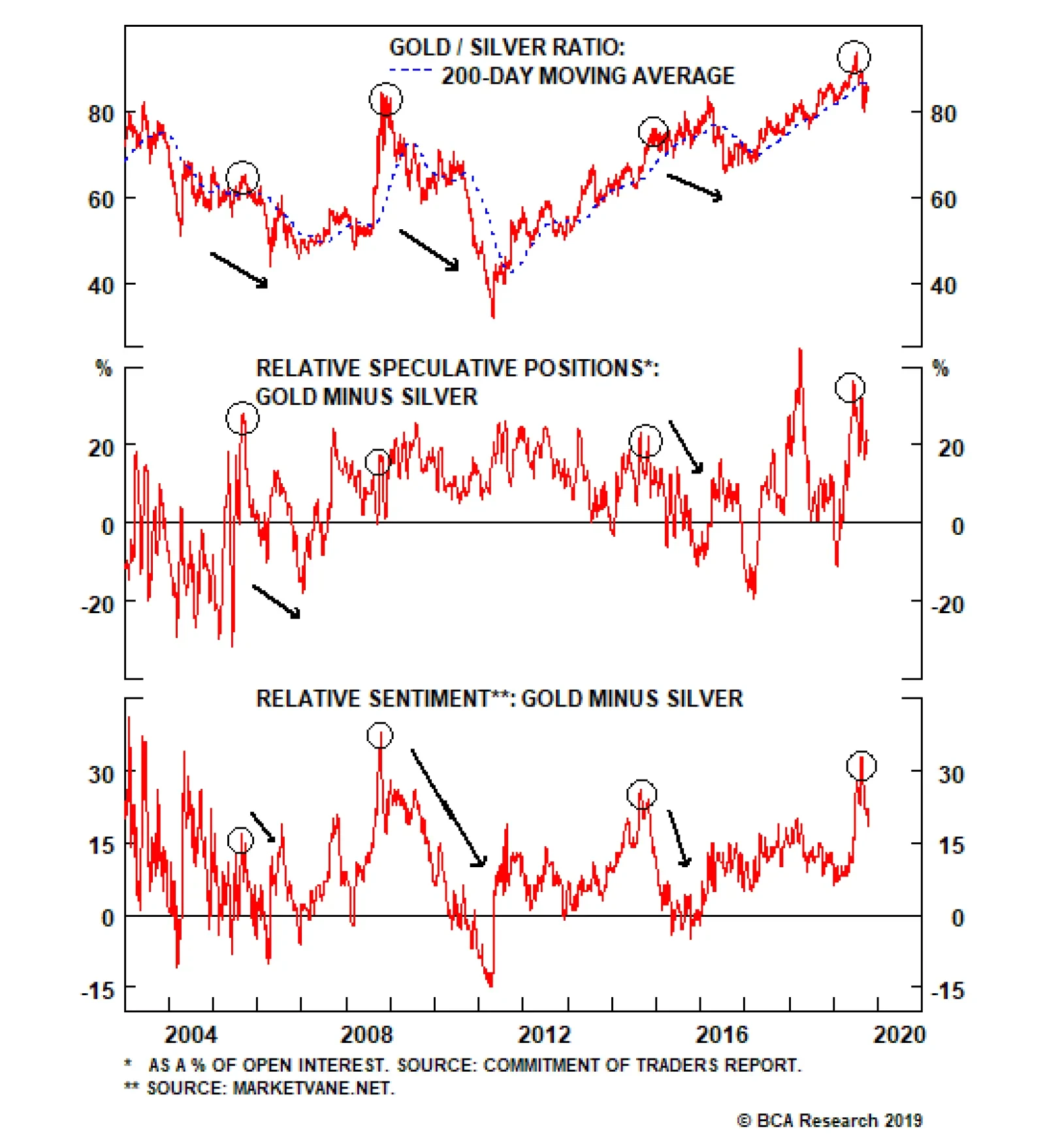
The gold/silver ratio (GSR) was in a race towards a major overhead resistance at 100 this summer, but after hitting a three-decade high of 93.3, it is now showing tentative signs of a reversal. Historically, these reversals tend to be powerful, quick, and…
Highlights The interim “phase 1” trade agreement reached last week represents a significant step forward towards reaching a détente in the China-U.S. trade war. Regardless of what happens next in the Brexit negotiations, a hard exit will be avoided. Stay long the pound. U.S. earnings growth is likely to be flat in the third quarter, in contrast to bottom-up expectations of a year-over-year decline. Earnings growth should pick up as global growth reaccelerates by year end. Stronger global growth will put downward pressure on the U.S. dollar. Remain overweight global equities relative to bonds over a 12-month horizon. Cyclical stocks should start to outperform defensives. Financials will finally have their day in the sun. Favorable Tradewinds In our Fourth Quarter Strategy Outlook published two weeks ago, we argued that global equities had entered a “show me” phase, meaning that tangible evidence of a de-escalation in the trade war and a recovery in global growth would be necessary for stock indices to move higher.1 We received some positive news on the trade front last Friday. In exchange for suspending the planned October 15th hike in tariffs from 25% to 30% on $250 billion of Chinese imports, China agreed to purchase $40-$50 billion of U.S. agricultural products per year, improve market access for U.S. financial services companies, and enhance the transparency of currency management. Admittedly, there is still much to be done. The text of the agreement has yet to be finalized. Both sides are aiming to conclude the deal by the time of the APEC summit in Santiago, Chile on November 16-17. Considering that a number of key issues remain unresolved, including what sort of enforcement and resolution mechanisms will be included in the deal, further delays or even a breakdown in the talks are possible. The interim deal agreed upon last week also punts the thorny issue of how to handle intellectual property protections to a “phase 2” of the negotiations slated to begin soon after “phase 1” is wrapped up. According to the independent and bipartisan U.S. Commission on the Theft of American Intellectual Property, U.S. producers lose between $225 and $600 billion annually from IP theft.2 China has often been considered among the worst offenders. Given the importance of the IP issue, meaningful progress will be necessary to ensure that tariffs of 15% on about $160 billion of Chinese imports are not introduced on December 15th. Trump Wants A Deal Despite the many hurdles that remain, last week’s developments significantly raise the prospects of a détente in the 18 month-long trade war. As a self-professed “master negotiator,” President Trump has put his credibility on the line by describing the negotiations as a “love fest,” calling the trade pact “the greatest and biggest deal ever made for our Great Patriot Farmers,” and saying that he has “little doubt” that a final agreement will be reached. Just as he did with NAFTA’s successor USMCA – a deal that is substantively similar to the one it replaced – Trump is likely to shift into marketing mode, trumpeting the “tremendous” new deal that he has negotiated on behalf of the American people. From a political point of view, this makes perfect sense. Rightly or wrongly, President Trump gets better marks from voters on his handling of the economy than anything else (Chart 1). A protracted trade war would undermine the U.S. economy, thereby hurting Trump’s re-election prospects. Chart 1Trump Gets Reasonably High Marks On His Handling Of The Economy, But Not Much Else
Kumbaya
Kumbaya
Chart 2Chinese Business Are Not Paying The Bulk Of The Tariffs
Kumbaya
Kumbaya
Notwithstanding his claims to the contrary, the evidence firmly suggests that U.S. consumers, rather than Chinese businesses, are paying the bulk of the tariffs. Chart 2 shows that U.S. import prices from China have barely declined, even as tariff rates on Chinese imports have risen. To the extent that the latest rounds of tariffs are focused on Chinese goods for which there is little U.S. or third-country competition, the ability of Chinese producers to pass on the cost of the tariffs will only increase. If all the tariff hikes that have been announced were implemented, the effective tariff rate on Chinese imports would rise from around 15% as of late August to as high as 25% in December (Chart 3). Such a tariff rate would reduce U.S. household disposable incomes by over $100 billion, wiping out most of the gains from the 2017 tax cuts. Trump can’t let the trade war reach this point. Chart 3Successive Rounds Of Tariffs Have Started To Add Up
Successive Rounds Of Tariffs Have Started To Add Up
Successive Rounds Of Tariffs Have Started To Add Up
Will China Play Hardball? One risk to a favorable resolution to the trade war is that China will increasingly see Trump as desperate to make a deal. This could lead the Chinese to take a hardline stance in the negotiations. While this risk cannot be dismissed, we would downplay it for three reasons: First, even though China’s exporters have been able to maintain some degree of pricing power during the trade war, trade volumes have still suffered, with exports to the U.S. down nearly 22% year-over-year in September. Second, as the crippling sanctions against ZTE have demonstrated, China remains highly dependent on U.S. technologies. This gives Trump a lot of leverage in the trade negotiations. Chart 4Who Will Win The 2020 Democratic Nomination?
Kumbaya
Kumbaya
Third, as Trump himself likes to say, China will find it easier to negotiate with him in his first term in office than in his second. Hoping that Trump would lose his re-election bid might have made sense for China a few months ago when Joe Biden was riding high in the polls; but now that Elizabeth Warren has emerged as the favorite to secure the Democratic nomination, that hope has been dashed (Chart 4). As we noted several weeks ago, China is likely to find Warren no less vexing on trade matters than Trump.3 All this suggests that China, just like Trump, will look for ways to cool trade tensions over the coming weeks. Brexit Breakthrough? As we go to press, the prospects for a Brexit deal have brightened. Although the details have yet to be released, the proposed deal would effectively put Northern Ireland in a veritable quantum superposition where it is both in the European common market and in the U.K. at the same time. This feat will be achieved by keeping Northern Ireland within the U.K. political jurisdiction but still aligned with EU regulatory standards. Negotiations could still go awry. Despite Prime Minister Boris Johnson’s assurance that he secured “a great new deal,” the Conservative’s coalition partner, the Northern Irish Democratic Unionist Party, is still withholding its support for the accord. Labour leader Jeremy Corbyn has also rejected the deal, saying that it is even worse than Theresa May’s originally proposed pact. Regardless of what transpires over the coming days, we continue to think that a hard Brexit will be avoided. Throughout the entire Brexit ordeal, we have argued that there was insufficient political support within the British ruling class for a no-deal Brexit. That conviction has only grown as polling data has revealed that an increased share of voters would choose to stay in the EU if another referendum were held (Chart 5). We have been long the pound versus the euro since August 3, 2017. The trade has gained 6.6% over this period. Investors should stick with this position. Based on real interest rate differentials, GBP/EUR should be trading near 1.30 rather than the current level of 1.16 (Chart 6). We expect the cross to move towards its fair value as hard Brexit risks diminish further. Chart 5Brexit Angst: A Case Of Bremorse
Brexit Angst: A Case Of Bremorse
Brexit Angst: A Case Of Bremorse
Chart 6Substantial Upside In The Pound
Substantial Upside In The Pound
Substantial Upside In The Pound
Global Growth Prospects Improving Chart 7Growth Slowdown Has Been More Pronounced In The Soft Data
Growth Slowdown Has Been More Pronounced In The Soft Data
Growth Slowdown Has Been More Pronounced In The Soft Data
Chart 8Manufacturing Output Rebounds Amid The ISM Slump
Manufacturing Output Rebounds Amid The ISM Slump
Manufacturing Output Rebounds Amid The ISM Slump
A détente in the trade war and a resolution to the Brexit saga should help support global growth. The weakness in the economic data has been much more pronounced in so-called “soft” measures such as business surveys than in “hard” measures such as industrial production (Chart 7). Notably, U.S. manufacturing output has stabilized over the past three months, even as the ISM manufacturing index has swooned (Chart 8). As sentiment rebounds, the soft data should improve. Global financial conditions have eased significantly over the past five months, thanks in large part to the dovish pivot by most central banks (Chart 9). The net number of central banks cutting rates generally leads the global manufacturing PMI by 6-to-9 months (Chart 10). In addition, the Fed’s decision to start buying Treasurys again will increase dollar liquidity, thus further contributing to looser financial conditions. Chart 9Easier Financial Conditions Will Boost Global Growth
Easier Financial Conditions Will Boost Global Growth
Easier Financial Conditions Will Boost Global Growth
Chart 10The Effects Of Easing Monetary Policy Should Soon Trickle Down To The Economy
The Effects Of Easing Monetary Policy Should Soon Trickle Down To The Economy
The Effects Of Easing Monetary Policy Should Soon Trickle Down To The Economy
Stepped-up Chinese stimulus should also help jumpstart global growth. Chinese money and credit growth both came in above expectations in September. The PBoC has been cutting reserve requirements, which has helped bring down interbank rates. Further cuts to the medium-term lending facility are likely over the remainder of this year. Changes in Chinese credit growth lead global growth by about nine months (Chart 11). Chart 11Chinese Credit Should Support The Recovery In Global Growth
Chinese Credit Should Support The Recovery In Global Growth
Chinese Credit Should Support The Recovery In Global Growth
Stay Overweight Global Equities While the road to finalizing a “phase 1” trade deal in time for the APEC summit is likely to be a bumpy one, we continue to reiterate our recommendation that investors overweight global stocks relative to bonds over a 12-month horizon. We expect to upgrade EM and European equities over the coming weeks once we see a bit more evidence that global growth is bottoming out. Ultimately, the trajectory of stocks will hinge on what happens to earnings. The U.S. earnings season began this week. As of last week, analysts expected S&P 500 EPS to decline by 4.6% in Q3 relative to the same quarter last year according to data compiled by FactSet. Keep in mind, however, that EPS growth has beaten estimates by around four percentage points since 2015 (Chart 12). Thus, a reasonable bet is that U.S. earnings will be flat this quarter, clearing a low bar of expectations. Chart 12Actual EPS Has Generally Beaten Estimates
Kumbaya
Kumbaya
Chart 13Earnings And Nominal GDP Growth Tend To Move In Lock-Step
Earnings And Nominal GDP Growth Tend To Move In Lock-Step
Earnings And Nominal GDP Growth Tend To Move In Lock-Step
The fact that 83% of the 63 S&P 500 companies that have reported earnings thus far have beaten estimates – better than the historic average of 64% – supports the view that current Q3 estimates are too dour. Looking out, earning growth should pick up as nominal GDP growth accelerates (Chart 13). European and EM equities generally outperform the global benchmark when global growth is speeding up (Chart 14). This is due to the more cyclical nature of their stock markets. In addition, as a countercyclical currency, the dollar tends to weaken in a faster growth environment. A weaker dollar disproportionately benefits cyclical stocks (Chart 15). Chart 14EM And Euro Area Equities Usually Outperform When Global Growth Improves
EM And Euro Area Equities Usually Outperform When Global Growth Improves
EM And Euro Area Equities Usually Outperform When Global Growth Improves
Chart 15Cyclical Stocks Will Outperform If The Dollar Weakens
Cyclical Stocks Will Outperform If The Dollar Weakens
Cyclical Stocks Will Outperform If The Dollar Weakens
We would include financials in our definition of cyclical sectors. As global growth improves, long-term bond yields will increase at the margin. Since central banks are in no hurry to raise rates, yield curves will steepen. This will boost bank profits and share prices (Chart 16). Cyclical stocks are currently quite cheap compared to defensives (Chart 17). Likewise, non-U.S. equities are quite inexpensive compared to their U.S. peers, even if one adjusts for differences in sector composition across regions. While U.S. stocks trade at 17.5-times forward earnings, international stocks trade at a more attractive forward PE ratio of 13.7. The combination of higher earnings yields and lower interest rates abroad implies that the equity risk premium is roughly two percentage points higher outside the United States (Chart 18). Chart 16Steeper Yield Curves Will Benefit Financials
Steeper Yield Curves Will Benefit Financials
Steeper Yield Curves Will Benefit Financials
Chart 17Cyclical Stocks Are More Attractive Than Defensives
Cyclical Stocks Are More Attractive Than Defensives
Cyclical Stocks Are More Attractive Than Defensives
Chart 18The Equity Risk Premium Is Quite High, Especially Outside The U.S.
The Equity Risk Premium Is Quite High, Especially Outside The U.S.
The Equity Risk Premium Is Quite High, Especially Outside The U.S.
We expect to upgrade EM and European equities over the coming weeks once we see a bit more evidence that global growth is bottoming out. Peter Berezin, Chief Global Strategist Global Investment Strategy peterb@bcaresearch.com Footnotes 1Please see Global Investment Strategy, “Fourth Quarter 2019 Strategy Outlook: A ‘Show Me’ Market,” dated October 4, 2019. 2 “Update to IP Commission Report: The Report of the Commission on the Theft of American Intellectual Property,” The National Bureau of Asian Research, 2017. 3Please see Global Investment Strategy Weekly Report, “Elizabeth Warren And The Markets,” dated September 13, 2019. Strategy & Market Trends MacroQuant Model And Current Subjective Scores
Kumbaya
Kumbaya
Strategic Recommendations Closed Trades
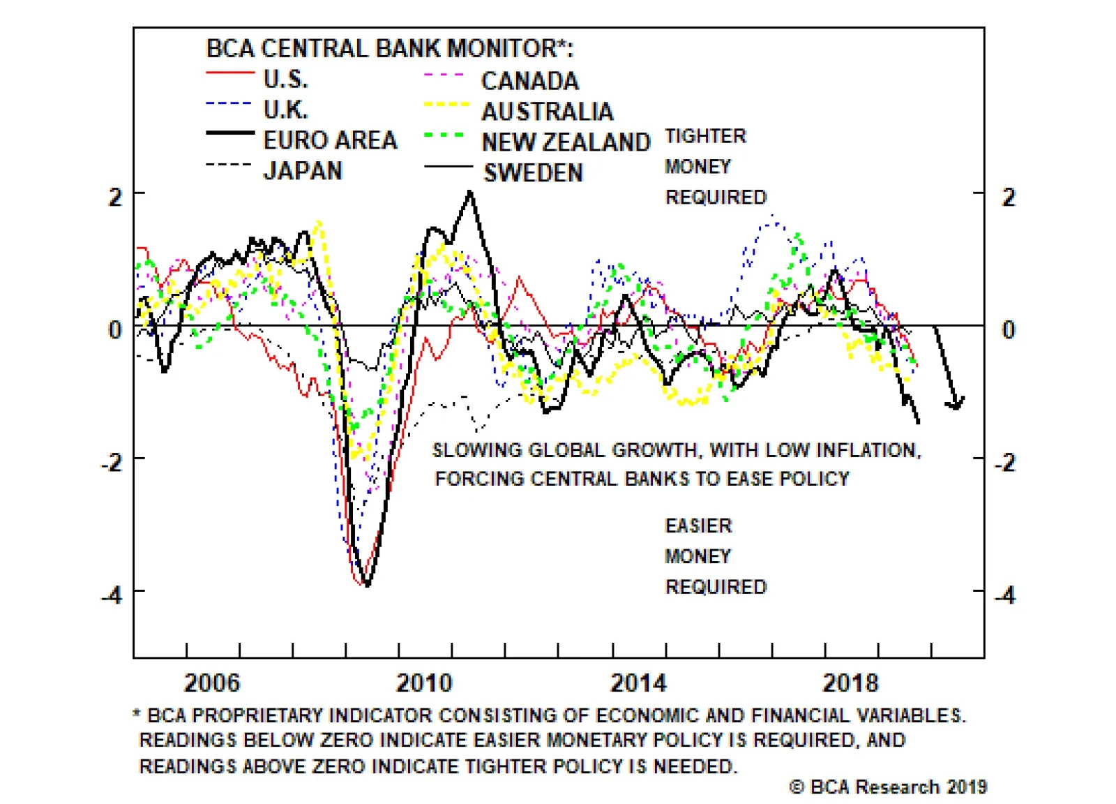
With the global manufacturing & trade downturn now threatening to spill over into domestic demand in the major advanced economies, policymakers will need to stay dovish to stave off a recession. This will keep global bond yields at depressed levels in the…
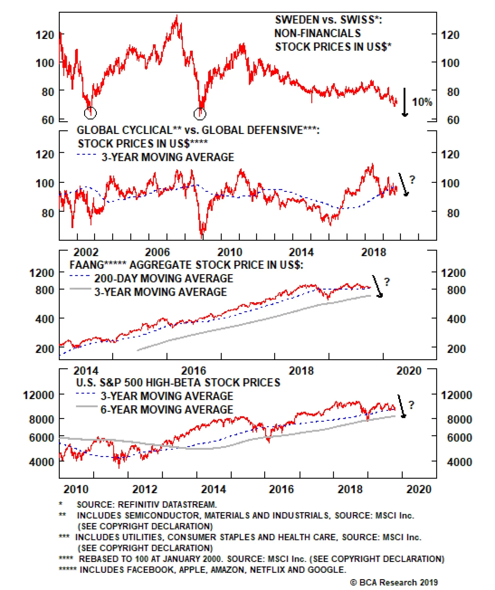
The ratio between Swedish and Swiss non-financial stocks in common currency terms is heading south. Swedish non-financials include many companies leveraged to the global industrial cycle, while Swiss non-financials are dominated by defensive stocks. Hence,…
Pervasive global policy uncertainty continues to fuel USD safe-haven demand. This keeps the Fed’s broad trade-weighted dollar index for goods close to record highs, which continues to stifle oil demand. At present, we do not expect this pervasive uncertainty to dissipate. For this reason, we are lowering our oil-demand growth expectation slightly for this year and next. Our estimate of global supply growth is slightly lower for this year and next, as well; we continue to expect OPEC 2.0 to maintain production discipline and for capital markets to restrain U.S. shale-oil growth.1 Our price forecast for 4Q19 is $66/bbl on average, an estimate that includes a risk premium reflecting continued tension in the Persian Gulf. Our updated supply-demand balances for 2020 reduce our Brent price forecast to $70/bbl versus our earlier expectation of $74/bbl. We continue to expect WTI to trade $4.00/bbl below Brent next year. Highlights Energy: Overweight. The Trump administration likely will not renew Chevron’s waiver to operate in Venezuela when it expires October 25. This raises the likelihood the country’s oil output will fall below 300k b/d, down from the 650k b/d we currently estimate.2 Production could revive next year, if Russian or Chinese firms step in to fill the void. This is not certain, however, as the U.S. is pressing both to end their support for the Maduro regime. Separately, the Aramco IPO could occur as early as November, according to press reports. Base Metals: Neutral. Copper treatment and refining charges in Asia are staging a recovery, clocking in at $56.70/MT at the end of last week, according to Metal Bulletin’s Fastmarkets. The MB index fell to a record low of $49.20/MT in late August. Precious Metals: Neutral. Gold volatility remains elevated – standing at 15.1% p.a. on the COMEX – as markets continue to process news re a partial easing of tensions in the Sino-US trade war. Geopolitical tensions, which now encompass Turkey-US relations, remain elevated. Ags/Softs: Underweight. Uncertainty around a partial deal involving ag exports from the U.S. to China remains high, as negotiators deliberately minimize expectations of a successful outcome. The big sticking point appears to be whether U.S. tariffs on Chinese imports due to kick in in December will be removed. Feature Uncertainty arising from global economic policy risk continues to dominate commodity markets. This has been the case going on three years. While it is ubiquitous, it is difficult to isolate. In earlier research, we noted the tightening of global financial conditions – largely the result of the Fed’s rates normalization policy, which resulted in four rate hikes last year, and China’s deleveraging policy – were responsible for the sharp slowing of oil demand seen in 2H18-1H19.3 Recently concluded research allows us to extend our earlier thesis to account for the effect of pervasive global policy uncertainty over the past three years, which has dominated our analysis of commodity markets generally, oil in particular. To wit: We find a strong, positive correlation between uncertainty, as measured by the Baker-Bloom-Davis Global Economic Policy Uncertainty (GEPU) index, and the Fed's USD broad trade-weighted index for goods (TWIBG) from January 2017 to now (Chart of the Week).4 Chart of the WeekUSD Absorbs Global Policy Uncertainty
USD Absorbs Global Policy Uncertainty
USD Absorbs Global Policy Uncertainty
USD Absorbs Global Uncertainty Sudden policy shifts have, over the past three years, resulted in a steady increase in the level of the GEPU index. Prior to 2017, the correlations between the GEPU index and the USD TWIBG were running at 33% and 63% for the periods 2000 to 2016 and 2010 to 2016, the post-GFC period for y/y returns. However, as right- and left-wing populism gained ground globally and monetary policy generally became more “data dependent” and ad hoc at the Fed, ECB and BoJ, the GEPU and USD TWIBG indices became highly correlated, surpassing 90% (Chart 2).5 This period saw the U.S. become more and more assertive vis-à-vis trade and foreign policy, particularly in re China, Iran and Venezuela, which caused those states to implement their own policy responses. In addition, as monetary policy generally became increasingly accommodative, central banks – and policy analysts – became less certain about the effects of their policies on the broader economy (e.g., the Fed shifting away from rates normalization, the ECB’s re-launching of QE, and the BoJ’s interest-rate targeting regime). Chart 2Co-Movement In GEPU, USD TWIBG
Co-Movement In GEPU, USD TWIBG
Co-Movement In GEPU, USD TWIBG
Often, commodity markets were forced to adjust to sudden policy changes – e.g., the imposition of trade tariffs against China, or the granting of waivers to Iran’s eight largest importers in November 2018 just before oil-export sanctions were re-imposed. Sudden policy shifts have, over the past three years, resulted in a steady increase in the level of the GEPU index. Increasing uncertainty translated into a steadily increasing USD TWIBG, with safe-haven demand for dollars rising, as the Chart of the Week indicates. To date, we have not decomposed the drivers of monetary conditions, particularly in re central-bank accommodation versus global economic policy uncertainty on the evolution of the USD. The GEPU index hit a record high in August 2019, while the USD TWIBG hit a record in September 2019. It is possible the effects of general policy uncertainty could be cumulative – as earlier uncertainties remain unresolved and new ones are added to the global mix (e.g., US-Turkey foreign-policy tensions now have been added to other geopolitical risks). It is entirely possible global monetary policy easing – particularly from the Fed – is accommodating safe-haven demand accompanying higher uncertainty. If the Fed were to tighten while uncertainty remains elevated the USD could rally sharply and impact commodity demand even more. Persistent USD Strength Lowers Oil Price Forecast Based on our analysis, the effects of the uncertainty we observe in the USD above are transmitted to GDP globally, which feeds through to commodity demand. As the USD strengthens, it raises the local-currency cost of commodities and the cost of servicing USD-denominated debt ex-US. In addition, on the supply side, a stronger dollar lowers local production costs at the margin, which stokes deflation globally. All else equal, these effects push oil prices lower by reducing demand and increasing supply at the margin. On the back of a stronger USD and persistent uncertainty, we are once again lowering our estimate of global demand growth. This is most pronounced in EM economies (Chart 3), but there are feedback effects into DM in the form of reduced trade volumes, which hits manufacturing economies like Germany harder than service-dominated economies like the US. On the back of a stronger USD and persistent uncertainty, we are once again lowering our estimate of global demand growth to 1.13mm b/d this year and 1.40mm b/d in 2020 (Chart 4). This is down slightly from 1.2mm b/d this year and 1.5mm b/d next year. In line with the U.S. EIA, we also lowered our estimate of 2018 demand, which has the effect reducing the level of demand we expect in 2019 and 2020. Chart 3Local-Currency Oil Costs Are High
Local-Currency Oil Costs Are High
Local-Currency Oil Costs Are High
Chart 4BCA Research Supply-Demand Balances
BCA Research Supply-Demand Balances
BCA Research Supply-Demand Balances
We maintain our expectation fiscal and monetary stimulus globally will revive demand, but, given the deleterious effects of global uncertainty and its effects on demand via the USD, we are moderating our position some, as the downward adjustment to consumption indicates. On the supply side, we expect KSA’s output to be fully restored by November, and for production in the Kingdom to average 9.9mm b/d in October and November. We are expecting overall OPEC 2.0 output growth of 250k b/d on average in the 2Q20 to 4Q20 interval, down from our previous growth estimate of 500k b/d. In the US, we expect shale-oil output to grow 900k b/d in 2020, versus 1.3mm b/d in 2019, which will leave overall U.S. crude output at 13.3mm b/d next year on average, as capital-market constraints continue to act as a governor on total output (Chart 5). Chart 5U.S. Shale-Oil Output Will Remain Capital-Constrained
U.S. Shale-Oil Output Will Remain Capital-Constrained
U.S. Shale-Oil Output Will Remain Capital-Constrained
Overall, we expect global supply to finish 2019 at 100.8mm b/d and at 102.3mm b/d next year, which is down slightly from our earlier estimates (Table 1). Even with demand moderating, we expect inventories to continue to draw this year and into 3Q20 before they resume building, as the combination of OPEC 2.0 production discipline and capital markets constrain output (Chart 6). Chart 6OECD Oil Inventories On Track To Draw
OECD Oil Inventories On Track To Draw
OECD Oil Inventories On Track To Draw
Table 1
Policy Uncertainty Lifts USD, Stifles Global Oil Demand Growth
Policy Uncertainty Lifts USD, Stifles Global Oil Demand Growth
Investment Implications Continued voluntary and involuntary production restraint will allow global inventories to draw despite slightly lower demand. Given our supply-demand expectations, we forecast Brent will trade lower next year, at $70/bbl on average versus our earlier expectation of $74/bbl. This is ~ $10/bbl above the median consensus. We continue to expect WTI to trade $4.00/bbl below Brent next year. Continued voluntary and involuntary production restraint will allow global inventories to draw despite slightly lower demand, which will keep Brent and WTI forward curves backwardated next year (WTI was in a slight carry earlier this week, while Brent was backwardated). We would caution that any resolution of the profound uncertainty currently dogging global markets could unleash pent-up demand that would sharply rally commodities generally, and oil in particular. This could take the form of a broad trade agreement that ends the Sino-US trade war – an unlikely, but not impossible, turn of events – or an unexpected reduction in tensions in the Persian Gulf, again, unlikely but not impossible. Bottom Line: Resolution of global policy uncertainty would revive commodity demand, as safe-haven USD demand gives way to higher consumer spending, renewed growth in global trade and investment. Until then, uncertainty will continue to hamper commodity demand growth, particularly for oil. Robert P. Ryan, Chief Commodity & Energy Strategist rryan@bcaresearch.com Hugo Bélanger, Senior Analyst Commodity & Energy Strategy HugoB@bcaresearch.com Footnotes 1 OPEC 2.0 is the moniker we coined for the producer coalition formed at the end of 2016 to regain control of production following the disastrous market-share war launched by OPEC in 2014, which took Brent prices from above $100/bbl to $26/bbl by early 2016. The coalition is led by the Kingdom of Saudi Arabia (KSA) and Russia. 2 Please see Venezuelan oil output could be halved without Chevron waiver extension: analysts, posted by S&P Global Platts October 14, 2019. 3 Please see our report entitle Central Bank Easing Key To Oil Prices, published September 5, 2019. It is available at ces.bcaresearch.com. 4 This GEPU is a monthly GDP-weighted index of newspaper headlines containing a list of words related to three categories – “economy,” “policy” and “uncertainty.” Newspapers from 20 countries representing almost 80% of global GDP (on an exchange-weighted basis) are scoured monthly to create the index. Please see GEPU and Baker-Bloom-Davis for additional information. 5 Both series are plotted as percent changes y/y in Chart 2. For the 2017 - 2019 period, the coefficient of determination for this model is 0.81 using a regression of the USD on the GEPU. There was no statistically significant relationship between them either from 2000 to 2016, or from 2010 to 2016. Insert SOFTS text here Investment Views and Themes Recommendations Strategic Recommendations Tactical Trades TRADE RECOMMENDATION PERFORMANCE IN 2019 Q3
Policy Uncertainty Lifts USD, Stifles Global Oil Demand Growth
Policy Uncertainty Lifts USD, Stifles Global Oil Demand Growth
Commodity Prices and Plays Reference Table Trades Closed in 2019 Summary of Closed Trades
Policy Uncertainty Lifts USD, Stifles Global Oil Demand Growth
Policy Uncertainty Lifts USD, Stifles Global Oil Demand Growth