Labor Market

Highlights The Eurostoxx600’s short bursts of outperformance require either global technology to underperform or the euro to underperform. EM’s short bursts of outperformance usually coincide with the global healthcare sector’s short bursts of underperformance. Remain tactically overweight to Europe and EM, but expect to reverse position later in the year. The ECB is justified in setting an accommodative monetary policy, but it is not justified in setting an ultra-accommodative monetary policy. Soft inflation prints will cap the extent to which bond yields can rise in the near term. Italian BTPs are an attractive long-term proposition, especially relative to other euro area bonds. Feature Chart of the WeekEuro Area Inflation Appears To Be Underperforming...
Euro Area Inflation Appears To Be Underperforming... ...But Adjusted For Its 'Negative Space' It Is Not
Euro Area Inflation Appears To Be Underperforming... ...But Adjusted For Its 'Negative Space' It Is Not
...But Adjusted For Its 'Negative Space' It Is Not
Euro Area Inflation Appears To Be Underperforming... ...But Adjusted For Its 'Negative Space' It Is Not
Euro Area Inflation Appears To Be Underperforming... ...But Adjusted For Its 'Negative Space' It Is Not
“The music is not in the notes, but in the silence between” – Wolfgang Amadeus Mozart As Mozart pointed out, true awareness lies not in appreciating what is there, but in appreciating what is not there. This is the concept of ‘negative space’: to understand an object, you have to understand the empty space that defines it. This week’s report extends the concept of negative space into the fields of investment and economics to make more sense of Europe’s recent past and its future. The Negative Space In Stock Markets Picking stock markets is a relative game. This means that what a stock market does not contain – its negative space – is often more important than what it does contain (Table I-1). This is not an abstract proposition, it is a mathematical truth. When a major global sector is strongly outperforming, a stock market’s zero or near-zero exposure to that sector will create a strong headwind to relative performance. And when the major sector is underperforming, its absence in the stock market will necessarily create a strong tailwind to relative performance.
Chart I-
For the European stock market, the negative space is technology, a sector in which European equities have a near-zero exposure. But there is another factor to consider: the currency. The technology sector’s global profits are mostly translated into shares quoted in dollars, while European equities’ global profits are mostly translated into shares quoted in euros. It follows that the Eurostoxx600’s short bursts of outperformance require at least one of the following two conditions (Chart I-2): Chart I-2The Eurostoxx600 Usually Outperforms When Technology Underperforms
The Eurostoxx600 Outperforms When Technology Underperforms
The Eurostoxx600 Outperforms When Technology Underperforms
Technology to underperform. Or: The euro to underperform. For emerging market (EM) equities, the negative space is healthcare, a sector in which EM has a near-zero exposure. Therefore unsurprisingly, EM’s short bursts of outperformance usually coincide with the healthcare sector’s short bursts of underperformance (Chart I-3). Sceptics will raise an obvious question: what is the cause and what is the effect? The answer is that sometimes EM is the driver of healthcare relative performance, and at other times vice-versa. Chart I-3EM Usually Outperforms When Healthcare Underperforms
EM Outperforms When Healthcare Underperforms
EM Outperforms When Healthcare Underperforms
A sharp slowdown emanating from emerging economies would undoubtedly drag down global equities. In the ensuing bear market, the more defensive healthcare sector would almost certainly outperform the financials. Under these circumstances the direction of causality would clearly be from EM to healthcare’s relative performance. On the other hand, absent a major bear market, in a common or garden reassessment of sector relative valuations versus their growth prospects, the causality would run in the other direction: sector rotation would drive the relative performance of equity markets: healthcare’s underperformance would help EM to outperform; and technology’s underperformance would help European equities to outperform. As we have explained in recent reports, the major sectors – and therefore the major stock markets – are now in this latter configuration in a brief countertrend burst before reverting to their structural trends later this year (Chart I-4 and Chart I-5). So for the time being, remain tactically overweight to Europe and to EM.1 Chart I-4The Eurostoxx600 Outperformance Is A Countertrend Burst
The Eurostoxx600 Outperformance Is A Countertrend Burst
The Eurostoxx600 Outperformance Is A Countertrend Burst
Chart I-5The EM Outperformance Is A Countertrend Burst
The EM Outperformance Is A Countertrend Burst
The EM Outperformance Is A Countertrend Burst
The Negative Space In European Inflation And Unemployment On the face of it, inflation is structurally underperforming in the euro area versus the U.S. But on closer examination this is only because of what the euro area harmonised index of consumer prices (HICP) does not contain: owner occupied housing costs – which tend to rise faster than other items in the price basket. Adjusting for this negative space in the HICP, the euro area and the U.S. have both achieved the exact same modest structural inflation, which their central banks define as ‘price stability’ (Chart of the Week). In a similar vein, the unemployment rate disregards changes in the labour participation rate. When people join the labour force – as they are in their tens of millions in Europe (Chart I-6) – the joining cohort tends to have a slightly higher unemployment rate given its inexperience in the formal labour market. So the joiners tend to lift the overall unemployment rate too. The paradox is that the percentage of the working age (15-74) population in employment also rises at the same time. Looking at this alternative measure of labour market health, the euro area employment market is in a structural uptrend and much healthier than it was at the peak of the last cycle in 2008 (Chart I-7). Chart I-6Europeans Are Joining The Labour Force In Their Tens Of Millions
Europeans Are Joining The Labour Force In Their Tens Of Millions
Europeans Are Joining The Labour Force In Their Tens Of Millions
Chart I-7The European Employment To Population Ratio Is In A Structural Uptrend
The European Employment To Population Ratio Is In A Structural Uptrend
The European Employment To Population Ratio Is In A Structural Uptrend
Hence, once we adjust for what is missing in euro area inflation and the euro area unemployment rate, neither inflation nor employment market performance appear to be too cold or too hot. This means that the ECB is justified in setting an accommodative monetary policy, but it is not justified in setting an ultra-accommodative monetary policy. The Negative Space In Monetary Policy The negative space in monetary policy is literally the negative space, by which we mean that interest rates cannot go deeply into negative territory. With the deposit rate already at -0.4 percent, the ECB’s room for manoeuvre in the dovish direction is limited. On the other hand, neither can monetary policy get meaningfully hawkish in the near term. The simple reason is that the ECB, like other central banks, is now even more wedded to ‘data-dependency’. The problem with this is that the data on which the central banks depend is always backward-looking. So policy will reflect what was happening one or two months ago, rather than what is happening now. Specifically, the plunge in the price of crude oil will depress both headline and core inflation rates (Chart I-8). And the recent wobble in risk-asset prices has weighed down some sentiment surveys (Chart I-9). Having promised to be data-dependent, the central banks have effectively created ‘an algorithm’ for their policy setting, an algorithm which everyone can see and read. It follows that the data, especially soft inflation prints, will cap the extent to which bond yields can rise in the near term. Chart I-8The Plunge In The Price Of Crude Will Subdue Inflation
The Plunge In The Price Of Crude Will Subdue Inflation
The Plunge In The Price Of Crude Will Subdue Inflation
Chart I-9The Stock Market Sell-Off Hurt Sentiment
The Stock Market Sell-Off Hurt Sentiment
The Stock Market Sell-Off Hurt Sentiment
However, core euro area bonds are an unattractive long-term proposition. When yields are so close to their lower bound, there is little scope for a capital gain, even in a crisis. Whereas the scope for a capital loss is considerably greater. By contrast, Italian BTPs are an attractive long-term proposition, especially relative to other euro area bonds. Almost all of the 2.75 percent yield on 10-year BTPs is a premium for euro break-up risk. Yet the populists in Italy do not want to break up the euro. And despite their rhetoric, neither do the populists in the core countries. To understand why, we must explain the negative space of ECB QE. When the ECB bought BTPs from Italian investors, what the Italian investors did not do was deposit the cash in Italian banks. Instead, they deposited it in German banks – something that we can see very clearly in the euro area’s mirror-image Target2 imbalances (Chart I-10). Chart I-10ECB QE Has Exacerbated The Target2 Imbalances
ECB QE Has Exacerbated The Target2 Imbalances
ECB QE Has Exacerbated The Target2 Imbalances
In effect, the core countries, through their equity in the Eurosystem, are holding a huge quantity of Italy’s €2.7 trillion of BTPs. Meaning that if the euro broke up, the core countries would be the ones picking up the tab. For the euro area’s future, this is the most important negative space of all. Dhaval Joshi, Senior Vice President Chief European Investment Strategist dhaval@bcaresearch.com Fractal Trading System* There are no new trades this week. But all four of our open trades – long PKR/INR, industrials versus utilities, litecoin and ethereum, and MIB versus Eurostoxx – are in profit. For any investment, excessive trend following and groupthink can reach a natural point of instability, at which point the established trend is highly likely to break down with or without an external catalyst. An early warning sign is the investment’s fractal dimension approaching its natural lower bound. Encouragingly, this trigger has consistently identified countertrend moves of various magnitudes across all asset classes. The post-June 9, 2016 fractal trading model rules are: When the fractal dimension approaches the lower limit after an investment has been in an established trend it is a potential trigger for a liquidity-triggered trend reversal. Therefore, open a countertrend position. The profit target is a one-third reversal of the preceding 13-week move. Apply a symmetrical stop-loss. Close the position at the profit target or stop-loss. Otherwise close the position after 13 weeks. Use the position size multiple to control risk. The position size will be smaller for more risky positions. * For more details please see the European Investment Strategy Special Report “Fractals, Liquidity & A Trading Model,” dated December 11, 2014, available at eis.bcaresearch.com Footnotes 1 Please see the European Investment Strategy Weekly Report, “Why 2019 Is The Mirror-Image Of 2018”, dated January 10, 2019, available at eis.bcaresearch.com. Fractal Trading Model Recommendations Asset Allocation Equity Regional and Country Allocation Equity Sector Allocation Bond and Interest Rate Allocation Currency and Other Allocation Closed Fractal Trades Trades Closed Trades Asset Performance Currency & Bond Equity Sector Country Equity Indicators Bond Yields Chart II-1Indicators To Watch - Bond Yields
Indicators To Watch - Bond Yields
Indicators To Watch - Bond Yields
Chart II-2Indicators To Watch - Bond Yields
Indicators To Watch - Bond Yields
Indicators To Watch - Bond Yields
Chart II-3Indicators To Watch - Bond Yields
Indicators To Watch - Bond Yields
Indicators To Watch - Bond Yields
Chart II-4Indicators To Watch - Bond Yields
Indicators To Watch - Bond Yields
Indicators To Watch - Bond Yields
Interest Rate Chart II-5Indicators To Watch - Interest Rate Expectations
Indicators To Watch - Interest Rate Expectations
Indicators To Watch - Interest Rate Expectations
Chart II-6Indicators To Watch - Interest Rate Expectations
Indicators To Watch - Interest Rate Expectations
Indicators To Watch - Interest Rate Expectations
Chart II-7Indicators To Watch - Interest Rate Expectations
Indicators To Watch - Interest Rate Expectations
Indicators To Watch - Interest Rate Expectations
Chart II-8Indicators To Watch - Interest Rate Expectations
Indicators To Watch - Interest Rate Expectations
Indicators To Watch - Interest Rate Expectations
Highlights Yield Curve Drivers: A rebound in rate hike expectations will cause the curve to steepen somewhat during the next few months, though accelerating wages limit the upside. The yield curve will not invert until after long-dated inflation expectations are fully re-anchored, probably not until late in the year. Yield Curve Positioning: Correlations that have been in place since the financial crisis show that the 5-year and 7-year maturities are most sensitive to changes in near-term rate hike expectations. With the discounter likely to move higher in the coming months, investors should favor yield curve trades that are short that portion of the curve. Investment Recommendation: Close our recommended long 2-year short 1-year/5-year trade for a profit of 2 bps. Replace it with a position short the 7-year bullet and long a duration-matched 2-year/30-year barbell. Feature The yield curve flattened throughout most of 2018, and actually fell enough that talk of curve inversion hit a fever pitch last November, around the same time that the market started to doubt the Fed’s ability to lift rates (Chart 1). As of today, the 2/10 Treasury slope sits at a mere 17 basis points, but we don’t see it falling below zero any time soon.1 Chart 1Too Soon For Curve Inversion
Too Soon For Curve Inversion
Too Soon For Curve Inversion
In this week’s report we consider the factors that will determine how the slope of the curve evolves over the next few months, and also recommend an investment strategy to take advantage of those movements. Yield Curve: Macro Drivers Driver 1: Rate Hike Expectations The number one factor that will influence the slope of the yield curve in the coming months is the market’s assessment of the near-term path for Fed rate hikes. Chart 2 shows the 5-year rolling correlation between monthly changes in the 2/10 slope and monthly changes in our 12-month Fed Funds Discounter. A positive correlation means that the 2/10 slope steepens when the market prices in more rate hikes and flattens when it prices in fewer hikes. A negative correlation means that the slope flattens when the market prices in more hikes and steepens when it prices in fewer hikes. Chart 2Rising Rate Expectations = Steeper 2/10 Slope
Rising Rate Expectations = Steeper 2/10 Slope
Rising Rate Expectations = Steeper 2/10 Slope
The correlation was consistently negative throughout the pre-crisis period because the 2-year yield reacted more to changes in near-term rate hike expectations than the 10-year yield. In other words, a given increase (decrease) in the discounter would lead to a larger increase (decrease) in the 2-year yield than in the 10-year yield, and the curve flattened (steepened) as a result. But this correlation flipped following the Great Recession. Zero-bound interest rates and Fed forward guidance were an important reason for the switch. But even during the past few months, as the 12-month discounter fell from 66 bps in early November to -1 bp currently, the 10-year yield fell by 45 bps and the 2-year yield by only 36 bps. Even with interest rates off zero and the Fed scaling back its forward guidance, the positive correlation between the 2/10 slope and the 12-month discounter persists. We think that the 12-month discounter is close to its near-term bottom. Our Fed Monitor has fallen somewhat in recent months but it remains above zero, suggesting that the economy requires further monetary tightening (Chart 3). A look at the three components of our Monitor gives us even more confidence that the discounter is near its trough. The economic growth component of the Monitor is nicely above zero (Chart 3, panel 3), and the inflation component continues to trend up (Chart 3, panel 4). All of the Fed Monitor’s recent weakness can be attributed to tighter financial conditions (Chart 3, bottom panel). As we discussed in last week’s report, now that the market views Fed policy as much more accommodative, it is only a matter of time before financial conditions ease.2 Chart 3Fed Monitor Still Suggests Tightening
Fed Monitor Still Suggests Tightening
Fed Monitor Still Suggests Tightening
In fact, some easing has already begun (Chart 4): Chart 4Financial Conditions Starting To Ease
Financial Conditions Starting To Ease
Financial Conditions Starting To Ease
The stock-to-bond total return ratio has bottomed (Chart 4, top panel) High-Yield spreads have peaked (Chart 4, panel 2) The VIX has moderated (Chart 4, panel 3) The trade-weighted dollar has started to depreciate (Chart 4, bottom panel) Ironically, easier financial conditions will give the Fed the green light to re-start rate hikes, probably by June, and this could re-test risk assets in the second half of the year. But between now and then, a move higher in 12-month rate expectations will apply some steepening pressure to the 2/10 slope. Driver 2: Inflation Expectations Instead of looking at nominal yields and rate hike expectations, another approach is to split yields into their real and inflation components. This is potentially revealing in the current environment since a large portion of the recent drop in yields was driven by the cost of inflation compensation. Since the November 8 peak in the discounter, the cost of 10-year inflation protection fell 26 bps and the real 10-year yield fell 19 bps. The cost of 2-year inflation protection declined 46 bps while the real 2-year yield actually rose 10 bps. Based on those numbers, it is evident that when the cost of inflation compensation fell alongside the oil price, it exerted a steepening pressure on the yield curve that was offset by a flattening in the real yield curve. One might conclude that a rebound in inflation will cause the curve to flatten going forward. That is probably true in the event of a pure inflation shock that does not impact global growth. But such a shock is highly unlikely. Oil (and other commodity) prices fell during the past few months because of a slowdown in global growth. A rebound in commodity prices that drives inflation higher will almost certainly occur alongside stronger global growth. In other words, splitting nominal yields into the real and inflation components probably doesn’t get us any closer to figuring out the near-term path for the yield curve. A better way to incorporate the cost of inflation compensation into our thinking about the yield curve is to focus on the 5-year/5-year forward TIPS breakeven inflation rate. That rate is currently 1.99%, well below the range of 2.3%-2.5% that has historically been consistent with well-anchored inflation expectations (Chart 5). Chart 5Inflation Expectations Are Too Low For The Fed
Inflation Expectations Are Too Low For The Fed
Inflation Expectations Are Too Low For The Fed
It is difficult to believe that the Fed would allow the yield curve to invert with the 5-year/5-year breakeven rate so low. The combination of an inverted yield curve and below-target inflation expectations would signal that the Fed wants to run a restrictive monetary policy before inflation has fully recovered. That would be completely contrary to the Fed’s mandate. From this argument, we reason that the 2/10 slope is unlikely to sustainably fall below zero until the 5-year/5-year forward TIPS breakeven rate is at least above 2.3%. With the 2/10 slope already at 17 bps, this means it is much more likely to stay near its current level or steepen somewhat during the next few months. Driver 3: Wage Growth The third factor driving our yield curve view is the pace of wage growth. Stronger wage growth is tightly correlated with a flatter yield curve, though the yield curve tends to lead wage growth by 6-12 months (Chart 6). Chart 6A Flatter Curve Leads Faster Wage Growth Higher Wage Growth = Flatter Curve
A Flatter Curve Leads Faster Wage Growth Higher Wage Growth = Flatter Curve
A Flatter Curve Leads Faster Wage Growth Higher Wage Growth = Flatter Curve
In fact, a typical cyclical pattern is for the 2/10 slope to flatten rapidly and then stay at a low (but positive) level for some time as wage growth catches up. In that sense, this cycle is playing out just like every other. The yield curve has already undergone its large flattening and wage growth is now accelerating to catch up. Bottom Line: The three factors discussed above lead us to expect a small amount of curve steepening during the next few months. A rebound in rate hike expectations due to easier financial conditions will cause the curve to steepen, though accelerating wages limit the upside. The yield curve will not invert until after long-dated inflation expectations are fully re-anchored, probably not until late in the year. Yield Curve Positioning In the first section of this report we noted that the 10-year yield fell by more than the 2-year yield between the early-November peak in the 12-month discounter and today. But Table 1 shows that the 5-year and 7-year yields fell by even more. This is the expected result. Table 1Treasury Curve From Peak In 12-Month Discounter To Present
Don't Position For Curve Inversion
Don't Position For Curve Inversion
Turning once again to the correlations between different segments of the yield curve and our 12-month discounter, we see that yield curve segments out to the 5-year maturity point are all positively correlated with the 12-month discounter. Also, curve segments beyond the 7-year maturity point are all negatively correlated with the discounter. The 5/7 slope has virtually no correlation (Chart 7). Chart 75-Year & 7-Year Are Most Sensitive To Rate Expectations
5-Year & 7-Year Are Most Sensitive To Rate Expectations
5-Year & 7-Year Are Most Sensitive To Rate Expectations
These correlations tell us that we should expect the 5-year and 7-year yields to move the most in response to changes in the 12-month discounter. In other words, if we expect the discounter to move higher in the coming months we should maintain short exposure to this part of the curve. This short exposure should be offset by long exposure at either the very short-end or the very long-end of the curve, where yields will see less upside when the discounter rebounds. To figure out where to focus this long exposure we can turn to our butterfly spread models.3 Table 2 presents the raw residuals from our butterfly spread models. These models are based on regressions of different butterfly spreads versus the slope of the yield curve segment that spans the two wings of the barbell portion of the trade. For example, Table 2 shows a residual of -9 bps for the 5-year bullet relative to the 2/10 barbell. This means that the 5-year appears 9 bps expensive versus the 2/10 barbell, given where the slope of the 2/10 curve is today. Table 3 shows the standardized residuals from the different curve models so that they can be compared against each other. Table 2Butterfly Strategy Valuation: Residuals
Don't Position For Curve Inversion
Don't Position For Curve Inversion
Table 3Butterfly Strategy Valuation: Standardized Residuals
Don't Position For Curve Inversion
Don't Position For Curve Inversion
Notice in Tables 2 and 3 that almost all of the numbers are negative. This means that bullet trades are currently expensive relative to barbell trades. Using our criteria of wanting to be short the 5-year or 7-year part of the curve, we can use the tables to see that a position short the 7-year bullet and long the duration-matched 2-year/30-year barbell has an attractive standardized residual of -1.00. This appears to be the most attractive curve trade for the current environment. As such, today we close our current yield curve recommendation to favor the 2-year bullet over the 1-year/5-year barbell for a gain of 2 bps. This recommendation had been in place since November 5. In its place, we initiate a recommendation to go long a duration-matched barbell consisting of the 2-year and 30-year maturities and short the 7-year note. Bottom Line: Correlations that have been in place since the financial crisis show that the 5-year and 7-year maturities are most sensitive to changes in near-term rate hike expectations. With the discounter likely to move higher in the coming months, investors should favor yield curve trades that are short that portion of the curve. With that in mind, we close our 2-year over 1-year/5-year trade and initiate a position short the 7-year bullet and long a duration-matched 2-year/30-year barbell. Ryan Swift, Vice President U.S. Bond Strategy rswift@bcaresearch.com Footnotes 1 We don’t expect to see sustained yield curve inversion until late this year. For further details please see U.S. Bond Strategy Special Report, “2019 Key Views: Implications For U.S. Fixed Income”, dated December 11, 2018, available at usbs.bcaresearch.com 2 Please see U.S. Bond Strategy Weekly Report, “Buy Corporate Credit”, dated January 15, 2019, available at usbs.bcaresearch.com 3 For further details on the models please see U.S. Bond Strategy Special Report, “More Bullets, Barbells And Butterflies”, dated May 15, 2018, available at usbs.bcaresearch.com Fixed Income Sector Performance Recommended Portfolio Specification
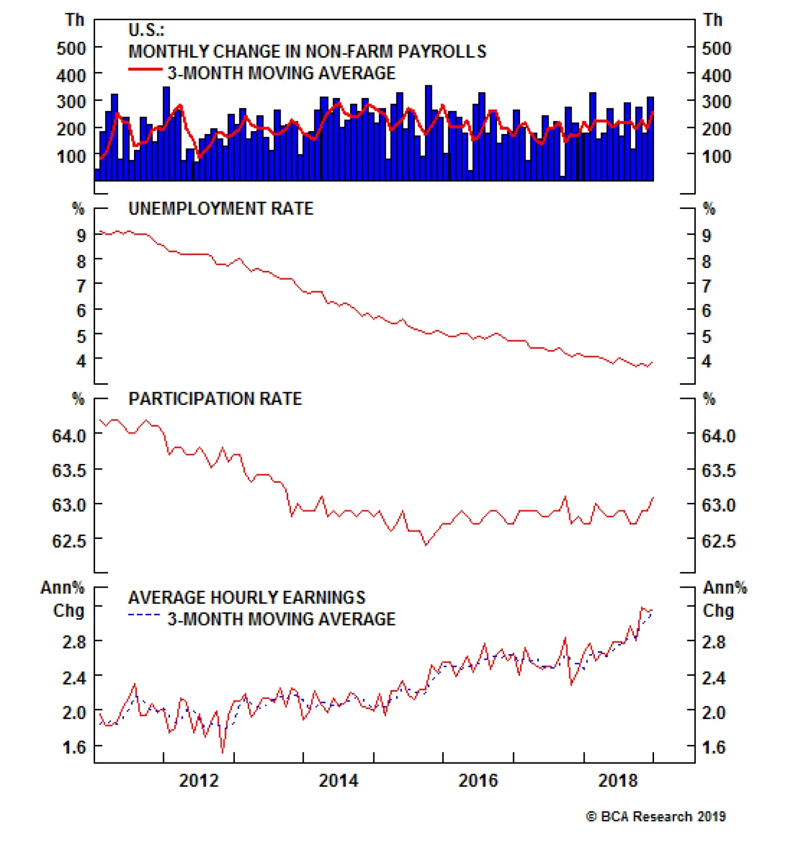
The December employment report pointed the way to an outcome that could satisfy financial markets and FOMC doves like Minneapolis president Kashkari. Despite the outsize expansion in nonfarm payrolls, the unemployment rate rose by two ticks because of a surge…
Highlights Survey data are easing, but that should not come as a surprise: The economy should decelerate as fiscal thrust is dialed back. Just a little patience (yeah-eah): A chorus of Fed speakers have taken to the podiums to reassure the public that the FOMC is taking its concerns seriously. The labor force participation rate popped in December, but investors shouldn’t count on it to produce a Goldilocks dual-mandate outcome: The demographic obstacle to continued part-rate gains is formidable. It is too early to de-risk portfolios: We remain constructive on risk assets and the economy. Feature Walking past flat-screen TVs during the workday has become considerably more pleasant. CNBC has switched out its red-drenched Market Sell-Off backdrop for a bright-green backdrop framing cheerful messages like, “Stocks are on track to rise for the third day in four.” In the ten sessions following Christmas Eve, the S&P 500 gained a stout 10%. Even a sharply negative preannouncement from Apple, and the prospect that 8% of Amazon’s outstanding shares could eventually hit the market, failed to halt the upward march. Only the disappointing December ISM Manufacturing survey has managed to bother the equity market over the course of the snapback rally, but the disappointment was quickly forgotten upon the next morning’s release of the gangbusters December employment report. The down-2.5%-one-day-up-3.5%-the-next action highlighted the fragility of the investor psyche. Markets are deeply uncertain about the economy, and how the Fed’s rate-hiking campaign will impact it. This week, we consider the evidence from the ISM and NFIB surveys, the recent wave of comments from Jay Powell and the regional Fed presidents, and the labor market to reassess our outlook for financial markets and the economy. Survey Says Over the first two weeks of January, the ISM surveys, the NFIB small business survey and the Job Openings and Labor Turnover Survey (JOLTS) all indicated slowing in their subject areas. An investor could point to them as evidence that the expansion is on its last legs, but we interpreted them as mixed, and do not see them as an argument for de-risking portfolios. Recall that the economy grew so far above trend in 2018 because of a generous helping of fiscal stimulus; as the stimulus is throttled back, the economy will decelerate. Markets had already factored the survey results into their expectations and took them in stride (Chart 1). Chart 1Soft Data Are Not A Surprise
Soft Data Are Not A Surprise
Soft Data Are Not A Surprise
The magnitude of the weakness in the manufacturing ISM survey did come as a surprise. Beneath the headline (Chart 2, top panel), the employment reading slipped (Chart 2, second panel) and prices paid plunged (Chart 2, third panel), suggesting that the economy may not be so robust after all, but at least stagflation is not yet a concern. New orders, the component with the best leading properties, fell a whopping eleven points to get uncomfortably close to the boom/bust line (Chart 2, bottom panel). Chart 2Manufacturing May Be Wobbling, ...
Manufacturing May Be Wobbling, ...
Manufacturing May Be Wobbling, ...
Manufacturing accounts for a modest share of U.S. employment and output, and we don’t dwell too much on it per se, but it may provide a window into global conditions. Trade tensions’ impact on global growth has been our foremost worry this year, and it is possible that the weakening manufacturing ISM points to weakness in the global economy. The U.S. is fairly inured from global weakness relative to other economies, but there is no such thing as decoupling. Weakness in the rest of the world will eventually make itself felt in the U.S., and we are watching the trade climate and global conditions carefully. The services ISM also declined more than expected, but a reading in the 57-58 range is strong, and points to an economy growing above trend. Employment (Chart 3, second panel) and new orders (Chart 3, bottom panel) both remain at or above a standard deviation above the mean. It is often true that markets care more about incremental changes than levels, but it is not an always-and-everywhere rule. In the context of an economy operating well above capacity, some slowing is both inevitable and desirable. We will watch the services ISM for signs of continued slowing, but we do not yet see any cause for concern. Chart 3... But Services Are Still Strong
... But Services Are Still Strong
... But Services Are Still Strong
Small-business optimism continues to support a constructive take on the economy, despite the modest pullback in the NFIB survey and some of its key components. The headline index has come off of the all-time highs it set in 2018, but remains at very high levels relative to history (Chart 4, top panel). Job openings hit an all-time high in December (Chart 4, second panel), underscoring the message from the persistently strong payrolls data, and the share of small businesses deeming it a good time to expand (Chart 4, third panel) and that plan to expand headcount over the next three months (Chart 4, bottom panel) are well above one-standard-deviation levels. Surveys are soft data, but both the headline optimism index and the good-time-to-expand component have begun to slide well in advance of the last three recessions, suggesting they’re useful leading indicators. Chart 4Small-Businesses Are Still Bulled Up
Small-Businesses Are Still Bulled Up
Small-Businesses Are Still Bulled Up
As strong as the employment picture has been, it is only a coincident indicator. The dot-com recession took employers (Chart 5, top panel) and job-hopping employees (Chart 5, bottom panel) by surprise, but there is nothing in the rate of job openings or quits in the JOLTS (Job Openings and Labor Turnover Survey) data that should inspire concern about the state of the economy. The series are off their highs, but there’s nothing to worry about at their still-elevated levels. Chart 5Softer, But Hardly Soft
Softer, But Hardly Soft
Softer, But Hardly Soft
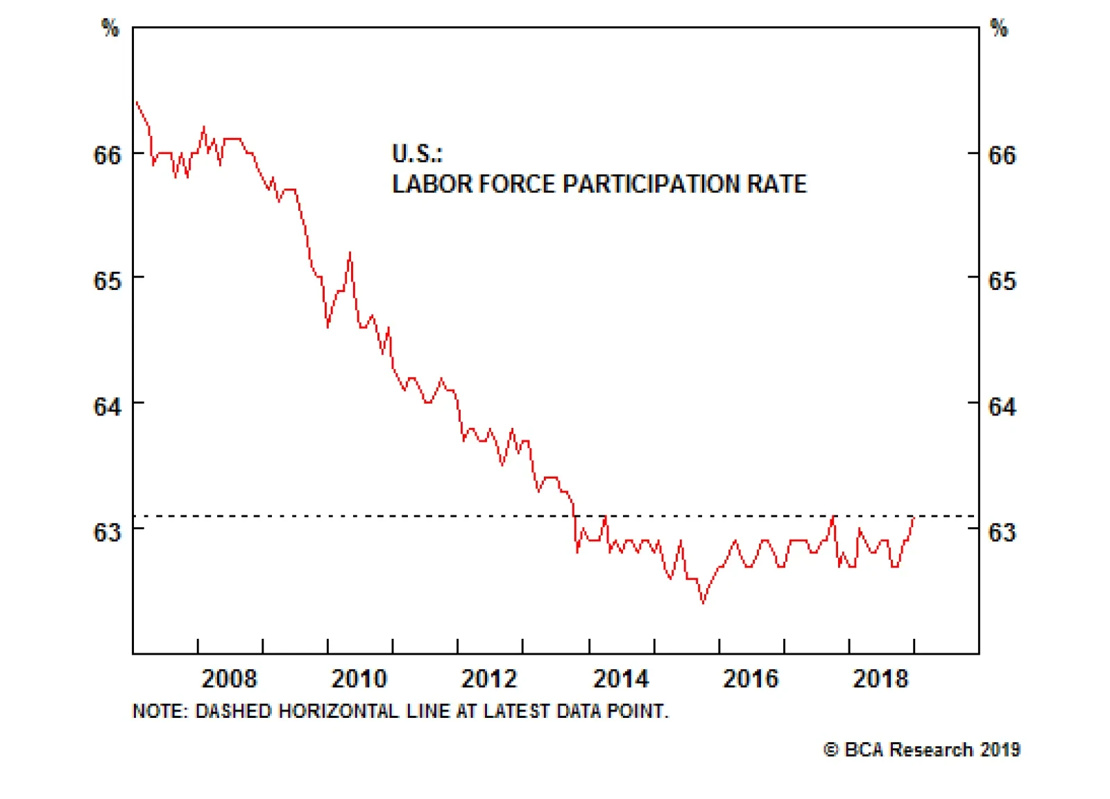
Bottom Line: Survey data have weakened as fiscal stimulus has waned, just as investors should have expected. We are keeping a close eye on the new orders component of the ISM Manufacturing survey, but nothing in the services ISM, NFIB or JOLTS surveys merits too much concern. FOMC Members Speak (And Speak, And Speak) The New Year brought an avalanche of comments from FOMC members. Chairman Powell, Vice Chairman Clarida, and seven regional presidents gave speeches, made appearances, or sat for interviews in the first two weeks of January, and New York Fed president Williams gave a long interview to CNBC two days after the December meeting. Away from uber-dove Bullard (St. Louis), who warned in a Wall Street Journal interview that further rate hikes could tip the economy into a recession, the various officials stressed the Fed’s open-mindedness. (Bullard, who is an FOMC voter this year, has repeatedly urged caution about hiking too much.) The overall thrust of the remarks has been to accentuate the FOMC’s commitment to go where the data lead. Echoing the language in the December minutes, several speakers noted that the Fed can be “patient,” given that inflation shows no signs of breaking out. The impact has been to soothe markets, which seem to be acutely concerned that rate hikes might go too far. (Though the speakers did little to ease concerns about balance-sheet reduction, or “quantitative tightening,” the Treasury, corporate-bond, and equity markets retraced much of their risk-off moves anyway.) Jay Powell set the tone for the overall message in a public appearance on January 4th, when he said the Fed “was listening sensitively to the message the markets are sending.” He underlined the data-dependency theme in an appearance last week, in which he said that, “we can be patient and flexible and wait and see what does evolve, and I think for the meantime, we’re waiting and watching. You should anticipate that we’re going to be patient and watching, and waiting and seeing.” His FOMC colleagues took care to drive home the same talking points, noting that data dependency includes following sentiment surveys, talking with business contacts, and watching markets. The speakers and the minutes also highlighted the discrepancy between robust 2018 growth of at least 3% and the much gloomier outlook implied by financial markets’ dreadful fourth quarter. None of the sensitive listeners disregarded the markets’ concerns, though Boston president Rosengren suggested that the markets may have gotten carried away. “My own view is that the economic outlook is actually brighter than the outlook one might infer from recent financial market movements.” Although we think the Fed will hike several more times before reaching this cycle’s terminal fed funds rate, the uniformity of the FOMC member comments leads us to expect that it will take a break, perhaps until June. Bottom Line: Our terminal fed funds rate estimate remains considerably higher than the money market’s, but we expect the Fed will pause for a few meetings. A pause may soothe markets and unwind the tightening of financial conditions that occurred in the fourth quarter, clearing the way for the Fed to resume its tightening campaign. Labor-Market Goldilocks The December employment report pointed the way to an outcome that could satisfy financial markets and FOMC doves like Minneapolis president Kashkari. Despite the outsize expansion in nonfarm payrolls, the unemployment rate rose by two ticks because of a surge in labor force participation. Last week, Kashkari attributed his ongoing aversion to rate hikes to the possibility that there’s more slack in the labor market than the committee may realize. “There might be a lot more people out there that we just don’t know [about] that are uncounted. Let’s go figure that out, and if we see inflationary pressures building, we can always hike rates then.” If the participation rate rises at a pace that allows new labor supply to offset continuing demand for workers, expanding payrolls don’t have to exert any generalized upward pressure on wages. Absent upward wage pressure, inflation could easily remain well-behaved. One month doesn’t make a trend, but December’s 63.1% reading brought the part rate back to the top of the range that has been in place for five years (Chart 6). A breakout could point the way to a Goldilocks outcome of inflation-free employment gains, but demographics suggest that there’s a limit to how much the part rate can advance. Chart 6Back To The Top Of The Range
Back To The Top Of The Range
Back To The Top Of The Range
The demographic drag on participation is largely a function of the baby boomers’ extended departure from the work force. AARP estimates that at least 10,000 of them turn 65 every day, and will continue to do so into the 2030s. Boomer employment was in its heyday in the late ‘90s, when potential participation exceeded 67% (Chart 7, top panel), and all of the baby boomers were in their prime working years.1 Now that they are exiting the labor force in a lengthy procession, labor force participation is swimming upstream, and it may not be able to do much more than hold the level it’s maintained since 2014. Chart 7How Much More Slack?
How Much More Slack?
How Much More Slack?
The shrinking supply of discouraged workers (workers who would start a job tomorrow if they were offered one, but are no longer actively looking for work and are therefore not counted as unemployed), suggests that much of the slack in the labor market has already been consumed (Chart 7, bottom panel). The disability rolls could be a source of Kashkari’s “uncounted” potential workers, however. The share of idled workers receiving disability benefits rose after the crisis (Chart 8), accounting for some of the widening gap between the part rate and the demographically-adjusted part rate. It is possible that some people who weren’t truly disabled will be motivated to come back to work, and their return to the work force may account for some of the pickup in participation, but our best guess is that they represent no more than a marginal source of labor supply. Chart 8Disability Claimants Won't Save The Day
Disability Claimants Won't Save The Day
Disability Claimants Won't Save The Day
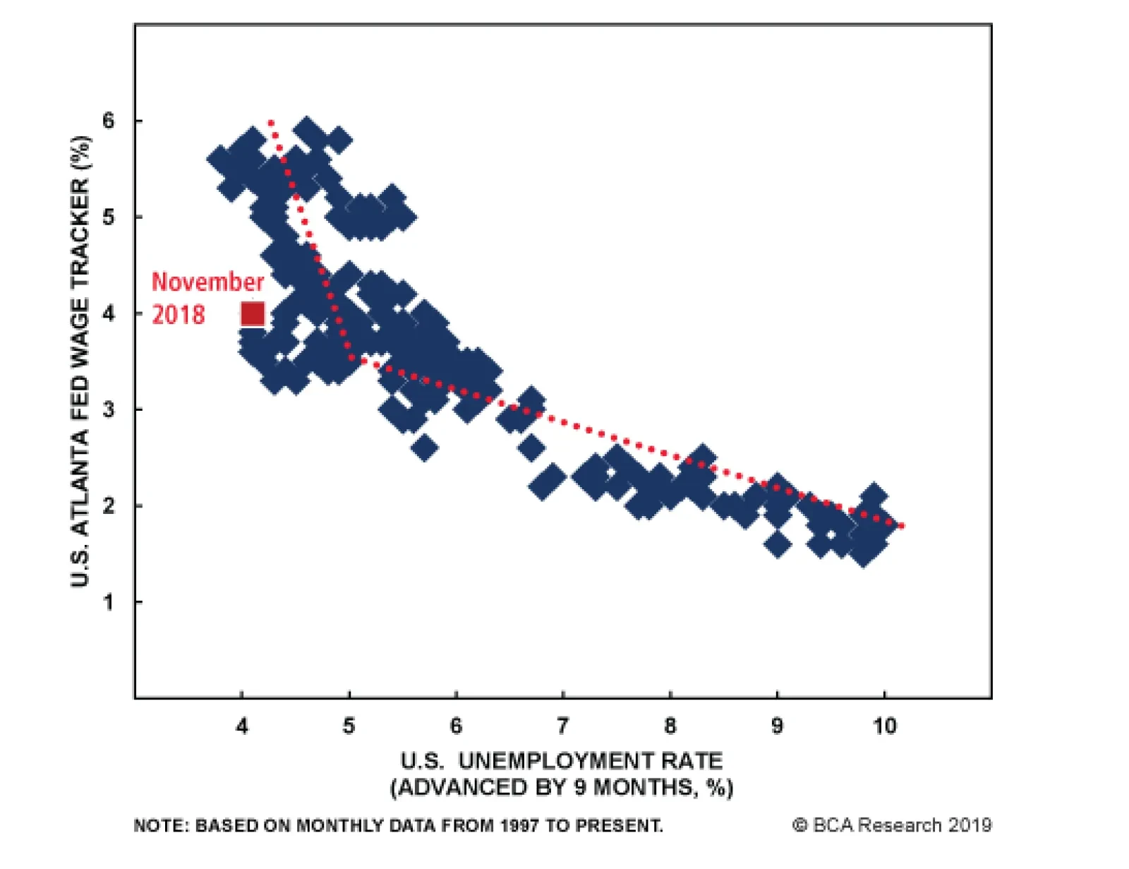
Bottom Line: The available evidence suggests that the labor market is quite tight. We expect that upward wage pressures will become increasingly apparent across 2019. Investment Implications An increasingly conciliatory Fed offers additional support for our equity overweight. A Fed pause might relieve some upward pressure on interest rates, but we expect that relief will only be temporary. As financial markets heal, easier financial conditions will clear the way for the Fed to resume its rate-hiking campaign. The sharp decline in Treasury yields at longer maturities only increases our conviction in underweighting Treasuries and maintaining below-benchmark duration positioning in all bond portfolios. As we noted last week, we think the high-yield bond market overreacted last quarter. Against a benign default outlook for 2019, 200 basis points of spread-widening seems extreme. A spread-product upgrade would fit with our equity upgrade, but we will wait until our U.S. Bond Strategy colleagues complete their review of their own recommendation before we consider changing our call. Doug Peta, Senior Vice President U.S. Investment Strategy dougp@bcaresearch.com Footnotes 1 Workers between the ages of 25 and 54, inclusive, are considered to be in their prime working years. The boomers were born between 1946 and 1964, and they were all in their prime working years from 1989 (when the youngest cohort turned 25) to 2000 (when the oldest cohort turned 54). 2018 was the last year that any of the boomers were between 25 and 54.
BCA has previously argued that the Phillips curve is “kinky” – that is it tends to be flat when unemployment is high, but to steepen sharply once unemployment falls below 5%. With the unemployment rate likely stuck below 4% for this year, wage growth will…
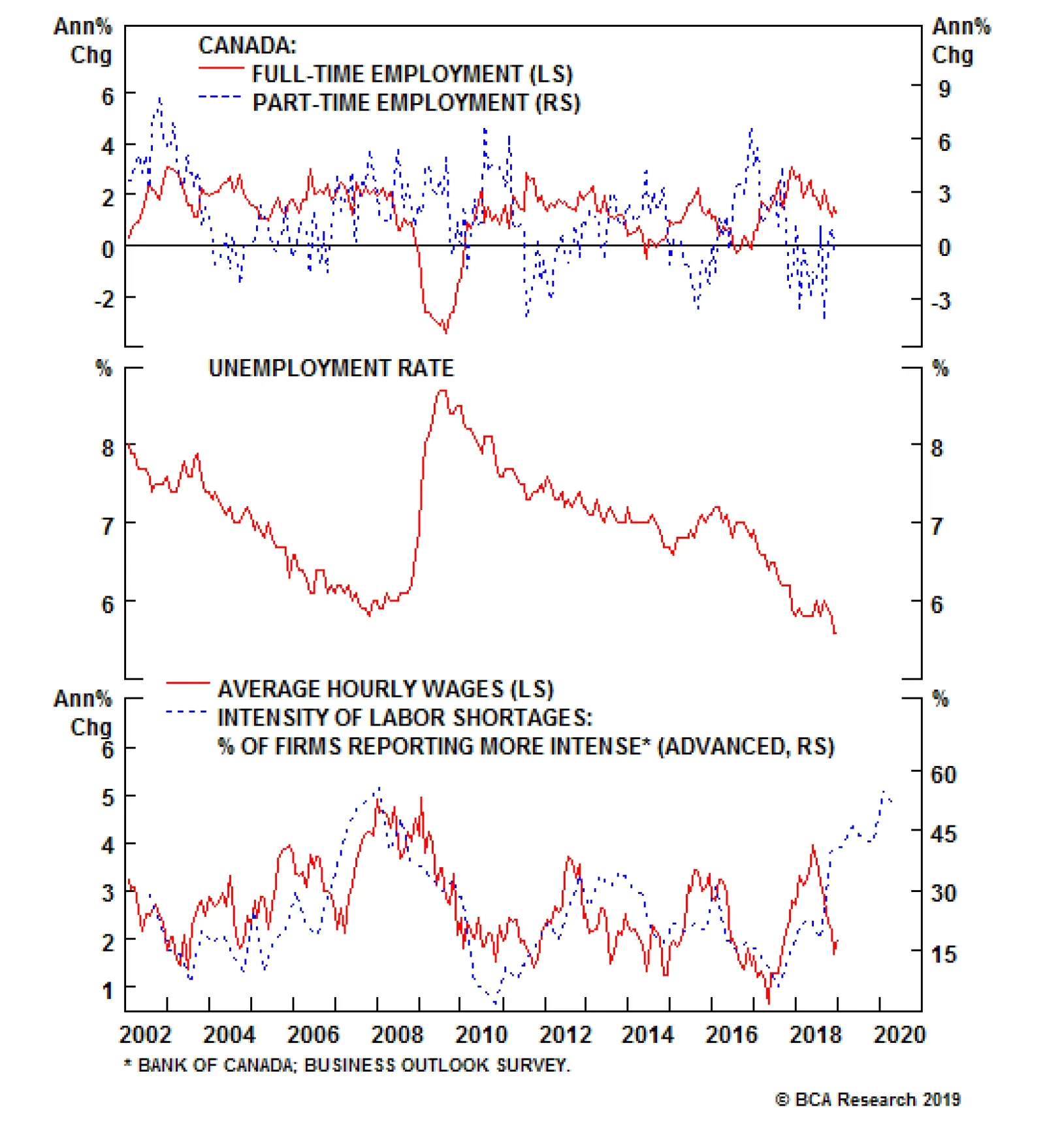
Unlike the very strong labor market conditions seen in the U.S. last December, the Canadian data came in slightly below expectations. Investors anticipated 10,000 Canadian jobs to be created in December against actual data of 9,300. But the headline…
We learned today that December marked a horrible month for risk assets, but a great month for the U.S. labor market. Caught in the crosscurrents between these opposing conditions of weakness and strength is the Fed. Elements of strength in the U.S. economy…
There are signs that the Chinese government is aiming to provide more support for less developed and urbanized parts of China. Beijing’s openness to rural-in-situ urbanization (i.e., urbanization without migration) suggests that the government is aiming to…
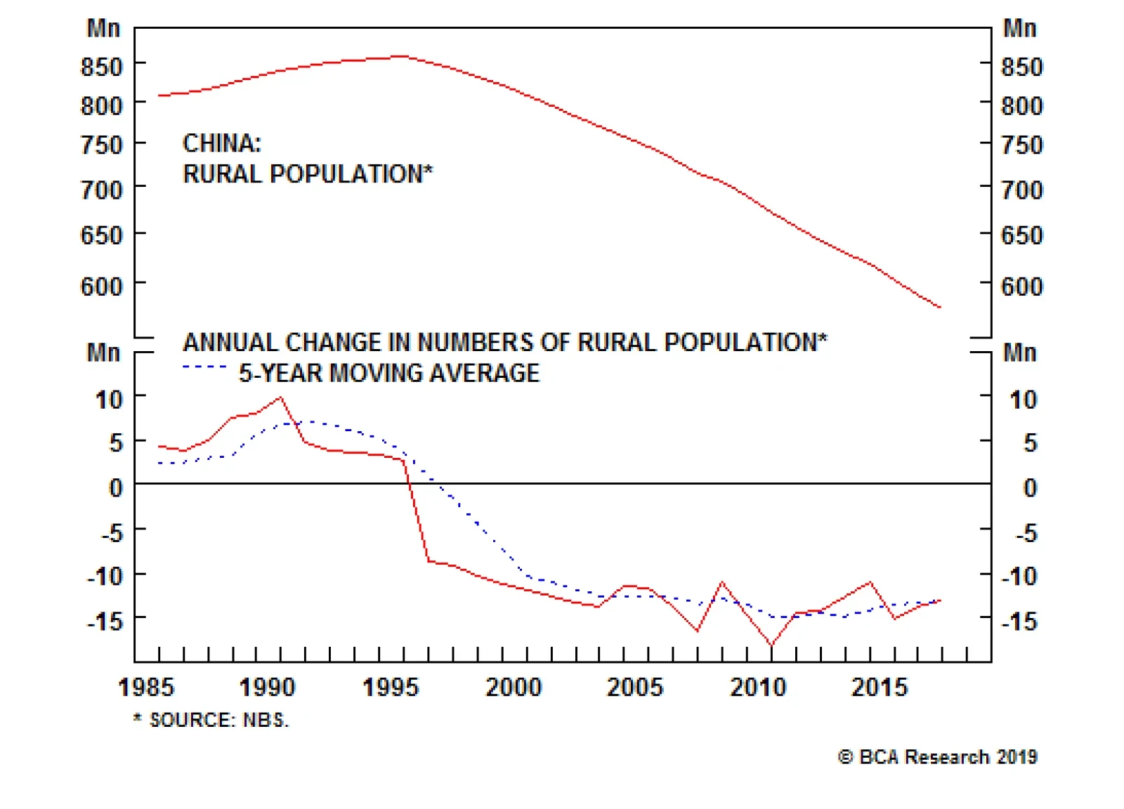
China’s rural population has declined by 33% from its peak of about 860 million in 1995 to 577 million in 2017 (see chart). All else equal, the lower rural population base alone will result in smaller rural-to-city migration compared to the previous two…
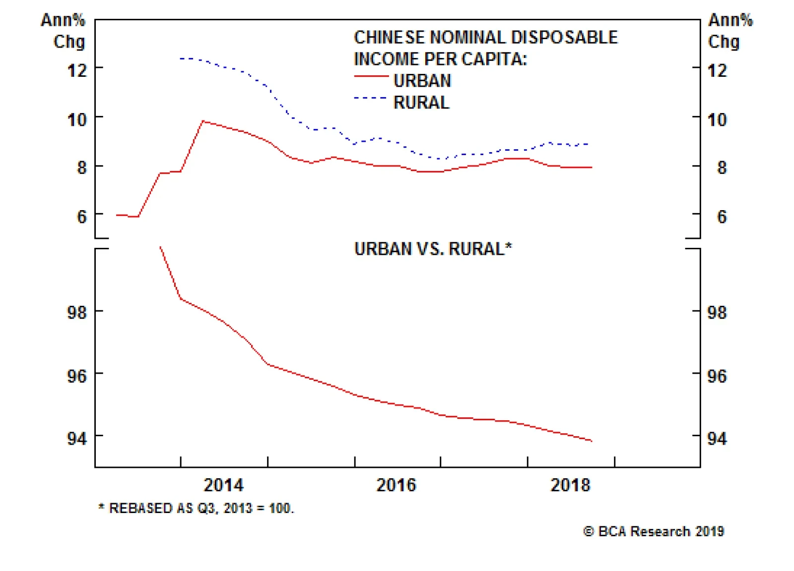
Our China strategists believe that the urbanization process will slow in China. There are several factors and trends that support their view on Chinese migration flows. First, rural-to-urban migration flows have already slowed in recent years. The number…